WIXLIB

by Misner, Thorne, and Wheeler, it is said that “Differential forms illuminate electromagnetic theory, andelectromagnetic theory illuminates differential forms” [40, 41]. In 1985, Feynman wrote that quantum electrodynamics (a superset of electromagnetic theory) had beenvalidated to be one of the most accurate equations to a few parts in a billion [42]. This is equivalent to anerror of a few human hair widths compared to the distance from New York to Los Angeles. More recently,Styer wrote in 2012 [43] that the accuracy had been improved to a few parts in a trillion [44]: such an erroris equivalent to a few human hair widths in the distance from the Earth to the Moon. More importantly, since Maxwell’s equations have been around for over 150 years, they have pervasivelyinfluenced the development of a large number of scientific technologies. This impact is particularly profoundin electrical engineering, ranging from rotating machinery, oil-gas exploration, magnetic resonance imaging,to optics, wireless and optical communications, computers, remote sensing, bioelectromagnetics, etc.Despite the cleaning up of Maxwell’s equations by Oliver Heaviside, he has great admiration for Maxwell asseen from his following statement [3], “A part of us lives after us, diffused through all humanity–more or less–andthrough all nature. This is the immortality of the soul. There are large souls and small souls. The immoral soul ofthe ‘Scienticulists’ is a small affair, scarcely visible. Indeed its existence has been doubted. That of a Shakespeareor Newton is stupendously big. Such men live the bigger part of their lives after they are dead. Maxwell is one ofthese men. His soul will live and grow for long to come, and hundreds of years hence will shine as one of the brightstars of the past, whose light takes ages to reach us.”3A Lone Simple Harmonic OscillatorElectromagnetic fields and waves can be thought of as a consequence of the coupling of simple harmonic oscillators.Hence, it is prudent first to study the physics of a lone harmonic oscillator, followed by analyzing a set of coupledharmonic oscillators. A lone harmonic oscillator can be formed by two masses connected by a spring, two moleculesconnected to each other by molecular forces, an electron trapped in a parabolic potential well, an electrical LCtank circuit, or even an electron-positron (e-p) pair bound to each other. The simplest description of the harmonicoscillator is via classical physics and Newton’s law. The inertial force of a mass is given by mass times acceleration,while the restoring force of the mass can be described by Hooke’s law. Hence, the equation of motion of a classical,simple harmonic oscillator ismd2q(t) κq(t)dt2(3.1)where m is the mass of the particle, q denotes the position of the particle,1 and κ is the spring constant. In thed2above, dt2 q(t) is the acceleration of the particle. The general solution to the above isq(t) b1 cos(Ωt) b2 sin(Ωt) b cos(Ωt θ)(3.2)pwhere Ω κ/m is the resonant frequency of the oscillator and b and θ are arbitrary constants. It has only onedcharacteristic resonant frequency. The momentum is defined as p(t) m dtq(t), and hence isp(t) mΩb1 sin(Ωt) mΩb2 cos(Ωt) mΩb sin(Ωt θ)4(3.3)A Lone Quantum Simple Harmonic OscillatorIn the microscopic regime, a simple harmonic oscillator displays quantum phenomena [8, 9, 48–53, 55]. Hence,the classical picture of the state of the particle being described by its position q and momentum p is insufficient.Therefore, in quantum mechanics, the state of the particle has to be more richly endowed by a wave function ψ(q, t).The motion of the wave function is then governed by Schrödinger equation.1qis used to denote position here as x is reserved for later use.3

Quantum mechanics cannot be derived: it was postulated, and the corresponding equation postulated bySchrödinger is [56] 2 2 V (q) ψ(q, t) i ψ(q, t)(4.1)22m q twhere V (q) 21 mΩ2 q 2 for the harmonic oscillator. The above is a parabolic wave equation (for a classification ofequations see [23, p. 527]) describing the trapping of a wave function (or a particle) by a parabolic potential well ofthe harmonic oscillator. The state of the particle is described by the wave function ψ(q, t). Once the wave functionis obtained by solving the above partial differential equation, then the position of the particle is obtain byZ dq ψ(q, t) 2 q hψ q ψi(4.2)hq(t)i where the angular brackets have been used to denote the expectation value of a random variable as in probability.The last equality follows from the use of Dirac notation [27] (also see Appendix in Part II). The wave function isnormalized such thatZ dq ψ(q, t) 2 1(4.3) Therefore, ψ(q, t) 2 P (q, t) can be thought of as a probability distribution function for the random variable q.And (4.2) can be thought of as the expectation value of q which is time varying because the wave function ψ(q, t)is time varying.The above is the recipé for determining the motion of a particle in quantum mechanics, and is an importantattribute of the probabilistic interpretation of quantum mechanics. Furthermore, the quantum interpretation impliesthat the position of the particle is indeterminate until after a measurement is made (see [8] for more discussion onquantum interpretation). Furthermore, the probabilistic interpretation implies that the position q and momentump are not deterministic quantities. They have a spread or standard deviation commensurate with their probabilisticdescription. This spread is known as the Heisenberg uncertainty principle [8, 9].To simplify the solution of Schrödinger equation, one can first solve for its eigenmodes, or assumes that themodal solution is time harmonic such that ψn (q, t) En ψn (q, t) t(4.4)ψn (q, t) ψn (q)e iωn t(4.5)i In other words, by the separation of variables,such that ωn En ; the eigenvalues have to be real for energy conservation or probability density conservation.Then (4.1) can be converted to a time independent ordinary differential equation 2 d212 2 mΩqψn (q) En ψn (q)(4.6)2m dq 22where En is its eigenvalue. These time independent solutions are known as stationary states because ψn (q, t) 2 Pn (q, t) ψn (q) 2 is time independent. The above equation has infinitely many closed-form eigensolutions dealtwith more richly in many text books (e.g., in [29–35]). It is important to note that the eigenvalues are given by 1En Ω n ωn(4.7)2with 1ωn Ω n 24(4.8)

It is to be noted that Ω is the natural resonant frequency of the harmonic oscillator, whereas ωn is the frequencyof the stationary state. Hence, in quantum theory, the harmonic oscillator can assume only discrete energy levels,En , and its energy can only change by discrete amount of Ω. This quantum of energy Ω is ascribed to that ofa single photon. For instance, quantum harmonic oscillator can change its energy level by absorbing energy fromits environment populated with photons, each carrying a packet of energy of Ω, or conversely, by the emission ofa photon. Even when n 0, implying the absence of photons (or zero field in the classical sense), En is not zero,giving rise to a fluctuating field which is the vacuum fluctuation of the field. Since this topic is extensively discussedin many text books [29–35], it will not be elaborated here.4.1Hamiltonian Mechanics Made SimpleSince quantum mechanics is motivated by Hamiltonian mechanics, the classical Hamiltonian mechanics will be firstreviewed. This mechanics is introduced in most textbooks by first introducing Lagrangian mechanics. Then theHamiltonian is derived from the Lagrangian by a Legendre transform [45]. In this paper, a simple way to arrive atthe Hamilton equations of motion will be given.The Hamiltonian represents the total energy of the system, expressed in terms of the momentum p and theposition q of a particle. For the lone harmonic oscillator, this Hamiltonian is given byH T V p2 (t) 1 2 κq (t)2m2(4.9)2(t)dHere, p(t) m dtq(t) is the momentum of the particle. The first term, T p2m, represents the kinetic energy of12the particle, while the second term, V 2 κq (t), is the potential energy of the particle: it is the energy stored inthe spring as expressed by Hooke’s law. In the above, p(t) and q(t) are independent variables. The Hamiltonian,representing total energy, is a constant of motion for an energy conserving system, viz., the total energy of such asystem cannot vary with time. Hence, p(t) and q(t) should vary with time t to reflect energy conservation. Takingthe first variation of the Hamiltonian with respect to time leads toδH H p H qδt δt 0 p t q t(4.10)In order for δH to be zero, one possibility is that H q , t p p H t q(4.11)The above equations are the Hamilton equations of motion.2 But the above equations are only determined to withina multiplicative constant, as δH is still zero when we multiply the right-hand side of both equations by a constant.This ambiguity follows from that a Hamiltonian which is multiplied by a constant is still a constant of motion.However, the constant can be chosen so that Newtonian mechanics is reproduced.Applying the Hamilton equations of motion yields qp , tm p κq t(4.12)The above can be combined to yield (3.1). These equations of motion imply that if p and q are known at a giventime, then time-stepping the above equations in the manner of finite difference time domain (FDTD) [46,47] method,their values at a later time can be obtained.The momentum and position can be normalized to yield a Hamiltonian of the formH 2 We could have used total derivatives foras time. q tand p t 1 2P (t) Q2 (t)2(4.13)but the these conjugate variables will later become functions of space as well5

where P (t) p(t)/ m, and Q(t) κq(t). With the use of (3.2) and (3.3), it can be shown that kinetic andpotential energies are time varying, but the sum of them is a constant implying energy conservation.An alternative representation is to factorize the above intoH 11 21P (t) Q2 (t) [iP (t) Q(t)] [ iP (t) Q(t)] B(t)B (t) (B(t)B (t) B (t)B(t))222(4.14)where B(t) iP (t) Q(t). If P (t) and Q(t) represent sinusoidal functions in quadrature phase, as seen in (3.2) and(3.3), then B(t) is now a complex rotating wave with a time dependence of e iΩt . Clearly, B(t)B (t) is independentof time, indicating that the Hamiltonian is a constant of motion.5Schrödinger Equation in Operator NotationThe Schrödinger equation in (4.1) can be formally written as [9, 55]Ĥ ψi i t ψi(5.1)where Ĥ is an operator in Hilbert space (an infinite dimensional vector space where the vectors have finite energyor norm, and the matrix operators that act on these vectors are also infinite dimensional). Here, ψi is a vector inHilbert space that Ĥ acts on. Furthermore,Ĥ T̂ V̂(5.2)where T̂ is the kinetic energy operator while V̂ is the potential energy operator. In order to conserve energy, theHamilton operator Ĥ, and the operators T̂ and V̂ , have to be Hermitian so that their eigenvalues are real. Theeigenvalues of Ĥ have to be real so that En in the previous section is real for energy conservation.For a general Schrödinger equation,p̂2,V̂ V (q̂)(5.3)T̂ 2mTo find the coordinate matrix representation of the above operator equation, one first defines a set of orthonormalvectors with the property that their inner product ishq q 0 i δ(q q 0 )(5.4)Furthermore, hq ψi ψ(q), namely, that the conjugate transpose vector hq has the sifting property that its innerproduct with the vector ψi yields a number that represents the value of the function ψ in the coordinate locationq. One further uses the definition of an identity operator [9, 55] (see also Appendix B in Part II)ZIˆ dq qihq (5.5)where qi is a set of orthonormal vectors. The above is a rather sloppy notation because q is used as an index ofthe vector qi as well as a position variable. And by the same token, qihq is an outer product of two vectors.By inserting the identity operator between Ĥ and ψi in (5.1), and testing the resulting equation with hq 0 , theabove equation (5.1) becomesZdqhq 0 Ĥ qihq ψi i t hq 0 ψi(5.6)Consequently, the coordinate matrix representation [9, 55], [23, p. 281] (see Appendix B of Part II) of the Hamiltonian operator ishq 0 Ĥ qi hq 0 T̂ qi hq 0 V̂ qi(5.7)Here, one assumes that the vector qi, indexed by the variable q, forms a complete orthonormal set, and the matrixrepresentation is the projection of the operator into the space spanned by the set of vectors qi.6

The coordinate matrix representations of these operators are (more discussions will be found in the Appendix,Part II) 2 2δ(q q 0 ),hq 0 V̂ qi δ(q q 0 )V (q)(5.8)hq 0 T̂ qi 2m q 2They are distribution functions, but they are often sloppily written asT̂ 2 2,2m q 2V̂ V (q)(5.9)These are often sloppily called the coordinate representations of these operators.If such representations of these operators are assumed, and identify that ψ(q) hq ψi, by inserting (5.8) into (5.6)then the equation postulated by Schrödinger in (4.1) is obtained. For a quantum harmonic oscillator, V̂ 21 mΩ2 q̂ 2 .In general,V̂ V (q̂)(5.10)where q̂ is the position operator. In the above, a function of an operator has meaning only when it is written as apower series or a Taylor expansion, and then acts on an eigenvector of the position operator q̂. For instance, f (q̂)has meaning only if it acts on an eigenvector of q̂, namely, qi. On that account,q̂ qi q qi,q̂ n qi q n qior thatf (q̂) qi [a0 a1 q̂ a2 q̂ 2 a3 q̂ 3 . . .] qi (a0 a1 q a2 q 2 a3 q 3 . . .) qi f (q) qi qif (q)ThenV (q̂) qi V (q) qi(5.11)It is clear from the above that functions of operators are themselves operators.The postulate for Schrödinger is also motivated by earlier proposition by de Broglie [57] that the momentum ofa particle is given by2πp k (5.12)λHence, for a plane wave function ψ(q) with exp(ikq) dependence representing the state of the particle, the momentumis expressible aspeikq keikq i q eikq i q ψ(q)(5.13)Therefore, the momentum operator in coordinate representation isp̂ i i q q(5.14)But the general momentum operator p̂ should be more appropriately written asp̂ i i q̂ q̂(5.15)The above derivative with respect to an operator has meaning only if it acts on a vector that is a function of theoperator q̂. Such a vector can be constructed by ψ1 i f (q̂) ψi. We can expand ψi in terms of the orthonormalbasis qi or simply let ψi qi, since the operator f (q̂) has meaning only if it acts on the eigenvector of theoperator q̂, namely, q̂ f (q̂) qi q f (q) qi qi q f (q). As a final note, Schrödinger equation was also motivated bythe findings of Planck [58] and the photoelectric effect [59, 60], which suggest that E Ω where E is the energyof a photon.7

6Schrödinger Picture versus Heisenberg PictureAt this juncture, it is prudent to discuss the difference between the Schrödinger picture versus the Heisenberg pictureof quantum mechanics [9, 48, 49, 51, 52]. In the Schrödinger picture, the time dependence is in the wavefunctionor the state vector ψi ψ(t)i; whereas in the Heisenberg picture, the time dependence is in the operator thatrepresents an observable which is a measurable quantity. As shall be seen, the Heisenberg picture is closer to theclassical picture.The formal solution to the Schrödinger equation (5.1) in operator form can be written asi ψ(t)i e Ĥt ψ0 i(6.1)where ψ0 i ψ(0)i is the state vector at t 0 which is independent of time, and Ĥ in (5.2) is time independent.The expectation value of an operator Ô, which represents an observable or a measurable quantity, isiihÔi hψ(t) Ô ψ(t)i hψ0 e Ĥt Ô e Ĥt ψ0 i hψ0 ÔH (t) ψ0 i(6.2)In the above, Ô is time independent in the Schrödinger picture, but ÔH (t) is time dependent in the Heisenbergpicture. Hence, in general, the relationship between an operator in the Schrödinger picture and in the Heisenbergpicture is given byiiÔH (t) e Ĥt ÔS e Ĥt(6.3)where the subscripts “H” and “S” mean the Heisenberg picture and the Schrödinger picture respectively. Clearly,ÔS ÔH (t 0). It can be shown easily that iihdÔHi Ĥ ÔH ÔH Ĥ Ĥ, ÔH dt (6.4)hiwhere Ĥ, ÔH Ĥ ÔH ÔH Ĥ is a commutator as defined by the above equation. This is the Heisenbergequation of motion for quantum operators. The commutator plays an important role in quantum mechanics: whentwo operators do not commute, or that their commutator is nonzero, then they cannot be determined preciselysimultaneously. More discussions can be found in standard quantum mechanics books [9, 55].6.1Quantum Hamiltonian MechanicsWe can derive the quantum version of Hamiltonian mechanics. In the Heisenberg picture, the operators whichrepresent observables are functions of time, and the equations of motion for the observable operators in Heisenbergpicture evolve asii q̂ih p̂ih q̂, Ĥ , p̂, Ĥ(6.5) t t The basic commutation relation is[q̂, p̂] q̂ p̂ p̂q̂ i Iˆ(6.6)Equation (6.6) above can be easily verified in the Schrödinger picture because the coordinate representations of p̂and q̂ arep̂ i q i , qq̂ q(6.7)Hence, (6.6) can be easily verified by substituting the above into it. In other words, they follow from de Broglieand Schrödinger postulates, which are the fundamental postulates leading to quantum mechanics. In contrast,some schools assume that the commutation relation [q̂, p̂] i Iˆ as the fundamental quantum postulate, and that8

de Broglie and Schrödinger postulates being derivable from it [8, 53]. Some authors refer to this as canonicalquantization, where the classical variables p and q as canonical variables that are elevated to be quantum operators,and the commutation relation between them as canonical commutation [52]. The two views are largely equivalent,but we favor the historical development over the formal commutation relation.Having verified (6.6) in Schrödinger picture, it can be easily verified in the Heisenberg picture as well, namely[q̂(t), p̂(t)] i Iˆ(6.8)(The above is also known as the equal time commutator.)It can be shown by the repeated application of the commutator in (6.6) that [52][p̂, q̂ n ] inq̂ n 1 (6.9)Note that the above is derived without applying calculus, but only using (6.8). Nevertheless we can borrow thecalculus notation and rewrite the above as nnn 1q̂(6.10)[p̂, q̂ ] inq̂ i q̂As mentioned earlier below (5.15), the derivative with respect to an operator has no meaning unless the operatoracts on its eigenvector. Consequently, the above can be rewritten as n n[p̂, q̂ n ] qi inq̂ n 1 qi inq n 1 qi i q qi i q̂ qi(6.11) q q̂In the above qi is the eigenvector of the position operator q̂ with eigenvalue q, namely, that q̂ qi q qi. It is to benoted that the q̂ operator above acts only on q̂ n , and nothing beyond to its right.One can expand3H(p̂, q̂) H0 (p̂, 0) H1 (p̂, 0)q̂ H2 (p̂, 0)q̂ 2 H3 (p̂, 0)q̂ 3 · · ·(6.12)hi p̂, Ĥ i H(p̂, q̂) q̂(6.13)i q̂, Ĥ i H(p̂, q̂) p̂(6.14)then it is clear thatSimilarly, one can show thathHence, (6.5) can then be rewritten as q̂ H(p̂, q̂) , t p̂ p̂ H(p̂, q̂) t q̂(6.15)The above are just the Hamilton equations for a quantum system: they bear striking similarities to the classicalHamilton equations of motion. It is clear from (6.12) that functions of operators are themselves operators. Hence,we neglect to put theˆabove the H in H(p̂, q̂) since they are obviously operators. It is to be noted that the aboveequations (6.15) do not involve , but surfaces in the coordinate representation of the operator p̂ in (6.7). Inaddition, one needs to take the expectation value of (6.15) to arrive at their classical analogue.Therefore, the procedure for obtaining the quantum equations of motion is clear. First, the classical Hamiltonianfor the system is derived. Then the conjugate variables, in this case, position q and momentum p, are elevatedto become quantum operators q̂ and p̂. In turn, the Hamiltonian becomes a quantum operator as well. Then thequantum equations of motion have the same algebra as the classical equations of motion as in (6.15). A summary3 Thisexpansion may not exist but for a Hamiltonian that is quadratic in p̂ and q̂, it exists.9

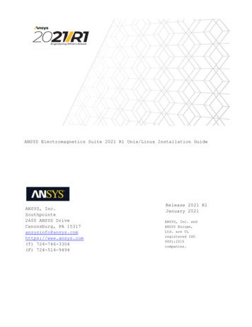
of this quantization procedure is given in Figure 1. This procedure and its modification are used mainly in thiswork.Very similar to (4.12), that eventually leads to (3.1), (3.2), and (3.3), it can be shown that for a quantumharmonic oscillator (see Appendix C in Part II for details),q̂(t) b̂1 cos(Ωt) b̂2 sin(Ωt),p̂(t) mΩb̂1 sin(Ωt) mΩb̂2 cos(Ωt)(6.16)Since q̂ and p̂ are operators representing observables in Heisenberg picture, they are time dependent and Hermitian.However, b̂1 and b̂2 are also Hermitian but time-independent, and not necessary commuting. It is to be remindedthese operators act on a state vector ψ0 i defined in (6.1). Hence, q̂(t) ψ0 i represents a new state vector of infinitedimension. With quantum interpretation, this indicates that the observable q̂ is probabilistic with infinite possiblevalues [8]. But its average value is given by hψ0 q̂(t) ψ0 i.Figure 1: (Left) The classical Hamiltonian and the classical equations of motion. (Right) The quantum Hamiltonianan

Quantum Electromagnetics: A New Look, Part I W. C. Chewy, A. Y. Liu, yC. Salazar-Lazaro, and W. E. I. Shaz September 20, 2016 at 16:04 Abstract Quantization of the electromagnetic eld has been