Transcription
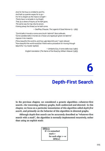
And, for the hous is crinkled to and fro,And hath so queinte weyes for to go—For hit is shapen as the mase is wroght—Therto have I a remedie in my thoght,That, by a clewe of twyne, as he hath goon,The same wey he may returne anoon,Folwing alwey the threed, as he hath come.— Geoffrey Chaucer, The Legend of Good Women (c. 8 )“Com’è bello il mondo e come sono brutti i labirinti!” dissi sollevato.“Come sarebbe bello il mondo se ci fosse una regola per girare nei labirinti,”rispose il mio maestro.[“How beautiful the world is, and how ugly labyrinths are,” I said, relieved.“How beautiful the world would be if there were a procedure for moving throughlabyrinths,” my master replied.]— Umberto Eco, Il nome della rosa ( 8 )English translation (The Name of the Rose) by William Weaver ( 8 )6Depth-First SearchIn the previous chapter, we considered a generic algorithm—whatever-firstsearch—for traversing arbitrary graphs, both undirected and directed. In thischapter, we focus on a particular instantiation of this algorithm called depth-firstsearch, and primarily on the behavior of this algorithm in directed graphs.Although depth-first search can be accurately described as “whatever-firstsearch with a stack”, the algorithm is normally implemented recursively, ratherthan using an explicit stack:DFS(v):if v is unmarkedmark vfor each edge v wDFS(w)
6. D -F S We can make this algorithm slightly faster (in practice) by checking whethera node is marked before we recursively explore it. This modification ensuresthat we call DFS(v) only once for each vertex v. We can further modify thealgorithm to compute other useful information about the vertices and edges,by introducing two black-box subroutines, P Vand PV, which weleave unspecified for now.DFS(v):mark vP V (v)for each edge vwif w is unmarkedparent(w)vDFS(w)P V (v)Recall that a node w is reachable from another node v in a directed graph G—or more simply, v can reach w—if and only if G contains a directed path from vto w. Let reach(v ) denote the set of vertices reachable from v (including vitself). If we unmark all vertices in G, and then call DFS(v), the set of markedvertices is precisely reach(v).Reachability in undirected graphs is symmetric: v can reach w if and onlyif w can reach v. As a result, after unmarking all vertices of an undirectedgraph G, calling DFS(v) traverses the entire component of v, and the parentpointers define a spanning tree of that component.The situation is more subtle with directed graphs, as shown in the figurebelow. Even though the graph is “connected”, different vertices can reachdifferent, and potentially overlapping, portions of the graph. The parentpointers assigned by DFS(v) define a tree rooted at v whose vertices areprecisely reach(v), but this is not necessarily a spanning tree of the graph.Figure 6. . Depth- rst trees rooted at different vertices in the same directed graph.As usual, we can extend our reachability algorithm to traverse the entireinput graph, even if it is disconnected, using the standard wrapper functionshown on the left in Figure . . Here we add a generic black-box subroutine 6
6. . Preorder and PostorderPPto perform any necessary preprocessing for the Pfunctions.VDFSA (G):P (G)for all vertices vunmark vfor all vertices vif v is unmarkedDFS(v)VandDFSA (G):P (G)add vertex sfor all vertices vadd edge s vunmark vDFS(s)Figure 6. . Two formulations of the standard wrapper algorithm for depth- rst searchAlternatively, if we are allowed to modify the graph, we can add a newsource vertex s, with edges to every other vertex in G, and then make a singlecall to DFS(s), as shown on the right of Figure . . Now the resulting parentpointers always define a spanning tree of the augmented input graph, but not ofthe original input graph. Otherwise, the two wrapper functions have essentiallyidentical behavior; choosing one or the other is entirely a matter of convenience.Again, this algorithm behaves slightly differently for undirected and directedgraphs. In undirected graphs, as we saw in the previous chapter, it is easy toadapt DFSA to count the components of a graph; in particular, the parentpointers computed by DFSA define a spanning forest of the input graph,containing a spanning tree for each component. When the graph is directed,however, DFSA may discover any number of “components” between 1 and V ,even when the graph is “connected”, depending on the precise structure of thegraph and the order in which the wrapper algorithm visits the vertices.6. Preorder and PostorderHopefully you are already familiar with preorder and postorder traversals ofrooted trees, both of which can be computed using depth-first search. Similartraversal orders can be defined for arbitrary directed graphs—even if they aredisconnected—by passing around a counter, as shown in Figure . . Equivalently, we can use our generic depth-first-search algorithm with the followingsubroutines P,P V, and PV.Pclock0(G):PV(v):clock clock 1v.pre clockPVclockv.post(v):clock 1clockThe equivalence of these two wrapper functions is a specific feature of depth-first search.In particular, wrapping breadth-first search in a for-loop to visit every vertex does not yield thesame traversal order as adding a source vertex and invoking breadth-first search at s.
6. D -F S DFSA (G):clock 0for all vertices vunmark vfor all vertices vif v is unmarkedclock DFS(v, clock)DFS(v, clock):mark vclock clock 1; v.pre clockfor each edge v wif w is unmarkedw.parentvclock DFS(w, clock)clock clock 1; v.post clockreturn clockFigure 6. . De ning preorder and postorder via depth- rst search.In either formulation, this algorithm assigns assigns v.pre (and advances theclock) just after pushing v onto the recursion stack, and it assigns v.post (andadvances the clock) just before popping v off the recursion stack. It follows thatfor any two vertices u and v, the intervals [u.pre, u.post] and [v.pre, v.post] areeither disjoint or nested. Moreover, [u.pre, u.post] contains [v.pre, v.post] if andonly if DFS(v) is called during the execution of DFS(u), or equivalently, if andonly if u is an ancestor of v in the final forest of parent pointers.After DFSA labels every node in the graph, the labels v.pre define apreordering of the vertices, and the labels v.post define a postordering of thevertices. With a few trivial exceptions, every graph has several different preand postorderings, depending on the order that DFS considers edges leavingeach vertex, and the order that DFSA considers vertices.For the rest of this chapter, we refer to v.pre as the starting time of v (orless formally, “when v starts”), v.post as the finishing time of v (or less formally,“when v finishes”), and the interval between the starting and finishing times asthe active interval of v (or less formally, “while v is active”).Classifying Vertices and EdgesDuring the execution of DFSA , each vertex v of the input graph has one ofthree states: new if DFS(v) has not been called, that is, if clock v.pre; active if DFS(v) has been called but has not returned, that is, if v.pre clock v.post; finished if DFS(v) has returned, that is, if v.post clock.Because starting and finishing times correspond to pushes and pops on therecursion stack, a vertex is active if and only if it is on the recursion stack. Itfollows that the active nodes always comprise a directed path in G.Confusingly, both of these orders are sometimes called “depth-first ordering”. Please don’tdo that. 8
6. . Preorder and Postorder12abcdefghijklmnopaebifngjcmhdlopk1 2 3 4 5 6 7 8 9 10 11 12 13 14 15 16 17 18 19 20 21 22 23 24 25 26 27 28 29 30 31 32Figure 6. . A depth- rst forest of a directed graph, and the corresponding active intervals of its vertices,de ning the preordering abfgchdlokpeinjm and the postordering dkoplhcgfbamjnie. Forest edges aresolid; dashed edges are explained in Figure 6. .The edges of the input graph fall into four different classes, depending onhow their active intervals intersect. Fix your favorite edge u v. If v is new when DFS(u) begins, then DFS(v) must be called during theexecution of DFS(u), either directly or through some intermediate recursivecalls. In either case, u is a proper ancestor of v in the depth-first forest, andu.pre v.pre v.post u.post.– If DFS(u) calls DFS(v) directly, then u v.parent and u v is called atree edge.– Otherwise, u v is called a forward edge. If v is active when DFS(u) begins, then v is already on the recursion stack,which implies the opposite nesting order v.pre u.pre u.post v.post.Moreover, G must contain a directed path from v to u. Edges satisfying thiscondition are called back edges. If v is finished when DFS(u) begins, we immediately have v.post u.pre.Edges satisfying this condition are called cross edges. Finally, the fourth ordering u.post v.pre is impossible.These edge classes are illustrated in Figure . . Again, the actual classificationof edges depends on the order in which DFSA considers vertices and the orderin which DFS considers the edges leaving each vertex.
6. D -F S sbackutreewscrossuttforwardtreevvforwardw1 2 3 4 5 6 7 8 9 10backcrossFigure 6. . Classi cation of edges by depth- rst search.Finally, the following key lemma characterizes ancestors and descendants inany depth-first forest according to vertex states during the traversal.Lemma . . Fix an arbitrary depth-first traversal of any directed graph G. Thefollowing statements are equivalent for all vertices u and v of G.(a)(b)(c)(d)u is an ancestor of v in the depth-first forest.u.pre v.pre v.post u.post.Just after DFS(v) is called, u is active.Just before DFS(u) is called, there is a path from u to v in which everyvertex (including u and v) is new.Proof: First, suppose u is an ancestor of v in the depth-first forest. Then bydefinition there is a path P of tree edges u to v. By induction on the pathlength, we have u.pre w.pre w.post u.post for every vertex w in P, andthus every vertex in P is new before DFS(u) is called. In particular, we haveu.pre v.pre v.post u.post, which implies that u is active while DFS(v) isexecuting.Because parent pointers correspond to recursive calls, u.pre v.pre v.post u.post implies that u is an ancestor of v.Suppose u is active just after DFS(v) is called. Then u.pre v.pre v.post u.post, which implies that there is a path of (zero or more) tree edges from u,through the intermediate nodes on the recursion stack (if any), to v.Finally, suppose u is not an ancestor of v. Fix an arbitrary path P from uto v, let x be the first vertex in P that is not a descendant of u, and let w bethe predecessor of x in P. The edge w x guarantees that x.pre w.post, andw.post u.post because w is a descendant of u, so x.pre u.post. It follows thatx.pre u.pre, because otherwise x would be a descendant of u. Because activeintervals are properly nested, there are only two possibilities: If u.post x.post, then x is active when DFS(u) is called. If x.post u.pre, then x is already finished when DFS(u) is called.
6. . Detecting CyclesWe conclude that every path from u to v contains a vertex that is not new whenDFS(u) is called.É6. Detecting CyclesA directed acyclic graph or dag is a directed graph with no directed cycles.Any vertex in a dag that has no incoming vertices is called a source; any vertexwith no outgoing edges is called a sink. An isolated vertex with no incidentedges at all is both a source and a sink. Every dag has at least one source andone sink, but may have more than one of each. For example, in the graph withn vertices but no edges, every vertex is a source and every vertex is a sink.abcdefghijklmnopFigure 6.6. A directed acyclic graph. Vertices e, f , and j are sources; vertices b, c , and p are sinks.Recall from our earlier case analysis that if u.post v.post for any edge u v,the graph contains a directed path from v to u, and therefore contains a directedcycle through the edge u v. Thus, we can determine whether a given directedgraph G is a dag in O(V E) time by computing a postordering of the verticesand then checking each edge by brute force.Alternatively, instead of numbering the vertices, we can explicitly maintainthe status of each vertex and immediately return Fif we ever discoveran edge to an active vertex. This algorithm also runs in O(V E) time; seeFigure . .I A(G):for all vertices vv.status Nfor all vertices vif v.status Nif I ADFS(v) Freturn Freturn TI ADFS(v):v.status Afor each edge v wif w.status Areturn Felse if w.status Nif I ADFS(w) Freturn Fv.statusreturn TFFigure 6. . A linear-time algorithm to determine if a graph is acyclic.
6. D -F S 6. Topological SortA topological ordering of a directed graph G is a total order on the verticessuch that uv for every edge u v. Less formally, a topological orderingarranges the vertices along a horizontal line so that all edges point from left toright. A topological ordering is clearly impossible if the graph G has a directedcycle—the rightmost vertex of the cycle would have an edge pointing to the left!On the other hand, consider an arbitrary postordering of an arbitrarydirected graph G. Our earlier analysis implies that u.post v.post for any edgeu v, then G contains a directed path from v to u, and therefore contains adirected cycle through u v. Equivalently, if G is acyclic, then u.post v.post forevery edge u v. It follows that every directed acyclic graph G has a topologicalordering; in particular, the reversal of any postordering of G is a topologicalordering of G.21a3bcdacdb4efgefjigmnho56ijkklhlpmjnmofpge1 2 3 4 5 6 7 8 9 10 11 12 13 14 15 16 17 18 19 20 21 22 23 24 25 26 27 28 29 30 31 32inoklphdcabFigure 6.8. Reversed postordering of the dag from Figure 6.6.If we require the topological ordering in a separate data structure, we cansimply write the vertices into an array in reverse postorder, in O(V E) time, asshown in Figure . .Implicit Topological SortBut recording the topological order into a separate data structure is usuallyoverkill. In most applications of topological sort, the ordered list of the verticesis not our actual goal; rather, we want to perform some fixed computation ateach vertex of the graph, either in topological order or in reverse topologicalorder. For these applications, it is not necessary to record the topological orderat all!
6. . Topological SortTTS(G):for all vertices vv.status NclockVfor all vertices vif v.status NclockTSDFS(v, clock):v.status Afor each edge v wif w.status NclockT Selse if w.status Afail gracefullyv.statusDFS(v, clock)SFS[clock]vclock clockreturn clockreturn S[1 . V]DFS(v, clock)1Figure 6. . Explicit topological sortIf we want to process a directed acyclic graph in reverse topological order,it suffices to process each vertex at the end of its recursive depth-first search.After all, topological order is the same as reversed postorder!PPP(G):for all vertices vv.status Nfor all vertices vif v is unmarkedPPDFS(v)PDFS(v):v.status Afor each edge v wif w.status NPPDFS(w)else if w.status Afail gracefullyv.status FP(v)If we already know that the input graph is acyclic, we can further simplify thealgorithm by simply marking vertices instead of recording their search status.PPD (G):for all vertices vunmark vfor all vertices vif v is unmarkedPPDPDFS(s)PD DFS(v):mark vfor each edge v wif w is unmarkedPPDP(v)DFS(w)This is just the standard depth-first search algorithm, with PVrenamedto P!Because it is such a common operation on directed acyclic graphs, I sometimesexpress postorder processing of a dag idiomatically as follows:PPD (G):for all vertices v in postorderP(v)
6. D -F S For example, our earlier explicit topological sort algorithm can be written asfollows:TS(G):clockVfor all vertices v in postorderS[clock]vclock clock 1return S[1 . V ]To process a dag in forward topological order, we can record a topologicalordering of the vertices into an array and then run a simple for-loop. Alternatively,we can apply depth-first search to the reversal of G, denoted rev(G), obtainedby replacing each each v w with its reversal w v. Reversing a directed cyclegives us another directed cycle with the opposite orientation, so the reversalof a dag is another dag. Every source in G is a sink in rev(G) and vice versa; itfollows inductively that every topological ordering of rev(G) is the reversal of atopological ordering of G. The reversal of any directed graph (represented in astandard adjacency list) can be computed in O(V E) time; the details of thisconstruction are left as an easy exercise.6. Memoization and Dynamic ProgrammingOur topological sort algorithm is arguably the model for a wide class of dynamicprogramming algorithms. Recall that the dependency graph of a recurrencehas a vertex for every recursive subproblem and an edge from one subproblemto another if evaluating the first subproblem requires a recursive evaluationof the second. The dependency graph must be acyclic, or the naïve recursivealgorithm would never halt.Evaluating any recurrence with memoization is exactly the same as performing a depth-first search of the dependency graph. In particular, a vertex of thedependency graph is “marked” if the value of the corresponding subproblem hasalready been computed. The black-box subroutines P Vand PVare proxies for the actual value computation. See Figure . .Carrying this analogy further, evaluating a recurrence using dynamic programming is the same as evaluating all subproblems in the dependency graph ofthe recurrence in reverse topological order—every subproblem is consideredafter the subproblems it depends on. Thus, every dynamic programming algorithm is equivalent to a postorder traversal of the dependency graph of itsunderlying recurrence!A postordering of the reversal of G is not necessarily the reversal of a postordering of G,even though both are topological orderings of G.
6. . Memoization and Dynamic ProgrammingM(x) :if value[x] is undefinedinitialize value[x]for all subproblems y of xM( y)update value[x] based on value[ y]finalize value[x]DFS(v) :if v is unmarkedmark vP V(x)for all edges v wDFS(w)PV(x)Figure 6. . Memoized recursion is depth- rst search. Depth- rst search is memoized recursion.DP(G) :for all subproblems x in postorderinitialize value[x]for all subproblems y of xupdate value[x] based on value[ y]finalize value[x]Figure 6. . Dynamic programming is postorder traversal.However, there are some minor differences between most dynamic programming algorithms and topological sort. First, in most dynamic programmingalgorithms, the dependency graph is implicit—the nodes and edges are notexplicitly stored in memory, but rather are encoded by the underlying recurrence. But this difference really is minor; as long as we can enumerate recursivesubproblems in constant time each, we can traverse the dependency graphexactly as if it were explicitly stored in an adjacency list.More significantly, most dynamic programming recurrences have highlystructured dependency graphs. For example, as we discussed in Chapter ,the dependency graph for the edit distance recurrence is a regular grid withdiagonals, and the dependency graph for optimal binary search trees is anupper triangular grid with all possible rightward and upward edges. Thisregular structure allows us to hard-wire a suitable evaluation order directly intothe algorithm, typically as a collection of nested loops, so there is no need totopologically sort the dependency graph at run time. We previously called thereverse topological order an evaluation order.Dynamic Programming in DagsConversely, we can use depth-first search to build dynamic programmingalgorithms for problems with less structured dependency graphs. For example,consider the longest path problem, which asks for the path of maximum totalweight from one node s to another node t in a directed graph G with weightededges. In general directed graphs, the longest path problem is NP-hard (by aneasy reduction from the traveling salesman problem; see Chapter ), but it is
6. D -F S Figure 6. . The dependency dag of the edit distance recurrence.easy to if the input graph G is acyclic, we can compute the longest path in G inlinear time, as follows.Fix the target vertex t, and for any node v, let LLP(v ) denote the Lengthof the Longest Path in G from v to t. If G is a dag, this function satisfies therecurrence LLP(v) 0if v t,max (v w) LLP(w) v w 2 Eotherwise,where (v w) denotes the given weight (“length”) of edge v w, and max ? 1. In particular, if v is a sink but not equal to t, then LLP(v) 1.The dependency graph for this recurrence is the input graph G itself:subproblem LLP(v) depends on subproblem LLP(w) if and only if v w is anedge in G. Thus, we can evaluate this recursive function in O(V E) time byperforming a depth-first search of G, starting at s. The algorithm memoizeseach length LLP(v) into an extra field in the corresponding node v.LP(v, t):if v treturn 0if v.LLP is undefinedv.LLP1for each edge v wv.LLP max v.LLP, (v w) Lreturn v.LLPP(w, t)In principle, we can transform this memoized recursive algorithm into adynamic programming algorithm via topological sort: 6
6. . Strong ConnectivityLP(s, t):for each node v in postorderif v tv.LLP 0elsev.LLP1for each edge v wv.LLP max v.LLP, (v w) w.LLPreturn s.LLPThese two algorithms are arguably identical—the recursion in the first algorithmand the for-loop in the second algorithm represent the “same” depth-firstsearch! Choosing one of these formulations over the other is entirely a matterof convenience.Almost any dynamic programming problem that asks for an optimal sequenceof decisions can be recast as finding an optimal path in some associated dag. Forexample, the text segmentation, subset sum, longest increasing subsequence,and edit distance problems we considered in Chapters and can all bereformulated as finding either a longest path or a shortest path in a dag, possiblywith weighted vertices or edges. In each case, the dag in question is thedependency graph of the underlying recurrence. On the other hand, “treeshaped” dynamic programming problems, like finding optimal binary searchtrees or maximum independent sets in trees, cannot be recast as finding anoptimal path in a dag.6. Strong ConnectivityLet’s go back to the proper definition of connectivity in directed graphs. Recallthat one vertex u can reach another vertex v in a directed graph G if G containsa directed path from u to v, and that reach(u) denotes the set of all verticesthat u can reach. Two vertices u and v are strongly connected if u can reach vand v can reach u. A directed graph is strongly connected if and only if everypair of vertices is strongly connected.Tedious definition-chasing implies that strong connectivity is an equivalencerelation over the set of vertices of any directed graph, just like connectivity inundirected graphs. The equivalence classes of this relation are called the stronglyconnected components—or more simply, the strong components—of G. Equivalently, a strong component of G is a maximal strongly connected subgraphof G. A directed graph G is strongly connected if and only if G has exactly onestrong component; at the other extreme, G is a dag if and only if every strongcomponent of G consists of a single vertex.The strong component graph scc(G) is another directed graph obtainedfrom G by contracting each strong component to a single vertex and collapsing
6. D -F S parallel edges. (The strong component graph is sometimes also called themeta-graph or condensation of G.) It’s not hard to prove (hint, hint) that scc(G)is always a dag. Thus, at least in principle, it is possible to topologically orderthe strong components of G; that is, the vertices can be ordered so that everyback edge joins two edges in the same strong component.abcdefghijklmnoabfgeijmncdhkloppFigure 6. . The strong components of a graph G and the strong component graph scc(G).It is straightforward to compute the strong component of a single vertex vin O(V E) time. First we compute reach(v) via whatever-first search. Thenwe compute reach 1 (v) {u v 2 reach(u)} by searching the reversal of G.Finally, the strong component of v is the intersection reach(v) \ reach 1 (v). Inparticular, we can determine whether the entire graph is strongly connected inO(V E) time.Similarly, we can compute all the strong components in a directed graphby combining the previous algorithm with our standard wrapper function.However, the resulting algorithm runs in O(V E) time; there are at most V strongcomponents, and each requires O(E) time to discover, even when the graph is adag. Surely we can do better! After all, we only need O(V E) time to decidewhether every strong component is a single vertex.6.6Strong Components in Linear TimeIn fact, there are several algorithms to compute strong components in O(V E)time, all of which rely on the following observation.Lemma . . Fix a depth-first traversal of any directed graph G. Each strongcomponent C of G contains exactly one node that does not have a parent in C.(Either this node has a parent in another strong component, or it has no parent.)Proof: Let C be an arbitrary strong component of G. Consider any path fromone vertex v 2 C to another vertex w 2 C. Every vertex on this path can reach w,and thus can reach every vertex in C; symmetrically, every node on this path canbe reached by v, and thus can be reached by every vertex in C. We concludethat every vertex on this path is also in C. 8
6.6. Strong Components in Linear TimeLet v be the vertex in C with the earliest starting time. If v has a parent,then parent(v) starts before v and thus cannot be in C.Now let w be another vertex in C. Just before DFS(v) is called, every vertexin C is new, so there is a path of new vertices from v to w. Lemma . nowimplies that w is a descendant of v in the depth-first forest. Every vertex on thepath of tree edges v to w lies in C; in particular, parent(w) 2 C.ÉThe previous lemma implies that each strong component of a directedgraph G defines a connected subtree of any depth-first forest of G. In particular,for any strong component C, the vertex in C with the earliest starting time is thelowest common ancestor of all vertices in C; we call this vertex the root of C.12abcdefghimjknolpabfgeinjchdmlokp1 2 3 4 5 6 7 8 9 10 11 12 13 14 15 16 17 18 19 20 21 22 23 24 25 26 27 28 29 30 31 32Figure 6. . Strong components are contiguous in the depth- rst forest.I’ll present two algorithms, both of which follow the same intuitive outline.Let C be any strong component of G that is a sink in scc(G); we call C a sinkcomponent. Equivalently, C is a sink component if the reach of any vertexin C is precisely C. We can find all the strong components in G by repeatedlyfinding a vertex v in some sink component (somehow), finding the verticesreachable from v, and removing that sink component from the input graph,until no vertices remain. This isn’t quite an algorithm yet, because it’s not clearhow to find a vertex in a sink component!SC(G):count 0while G is non-emptyC?count count 1vany vertex in a sink component of Gfor all vertices w in reach(v)w.label countadd w to Cremove C and its incoming edges from GhhMagic!iiFigure 6. . Almost an algorithm to compute strong components.
6. D -F S Kosaraju and Sharir’s AlgorithmAt first glance, finding a vertex in a sink component quickly seems quite difficult.However, it’s actually quite easy to find a vertex in a source component—a strongcomponent of G that corresponds to a source in scc(G)—using depth-first search.Lemma . . The last vertex in any postordering of G lies in a source componentof G.Proof: Fix a depth-first traversal of G, and let v be the last vertex in the resultingpostordering. Then DFS(v) must be the last direct call to DFS made by thewrapper algorithm DFSA . Moreover, v is the root of one of the trees inthe depth-first forest, so any node x with x.post v.pre is a descendant of v.Finally, v is the root of its strong component C.For the sake of argument, suppose there is an edge x y such that x 62 Cand y 2 C. Then x can reach y, and y can reach v, so x can reach v. Because vis the root of C, vertex y is a descendant of v, and thus v.pre y.pre. The edgex y guarantees that y.pre x.post and therefore v.pre x.post. It followsthat x is a descendant of v. But then v can reach x (through tree edges),contradicting our assumption that x 62 C.ÉIt is easy to check (hint, hint) that rev(scc(G)) scc(rev(G)) for any directedgraph G. Thus, the last vertex in a postordering of rev(G) lies in a sink componentof the original graph G. Thus, if we traverse the graph a second time, where thewrapper function follows a reverse postordering of rev(G), then each call to DFSvisits exactly one strong component of G.Putting everything together, we obtain the algorithm shown in Figure . ,which counts and labels the strong components of any directed graph in O(V E)time. This algorithm was discovered (but never published) by Rao Kosarajuin, and later independently rediscovered by Micha Sharir in. TheKosaraju-Sharir algorithm has two phases. The first phase performs a depth-firstsearch of rev(G), pushing each vertex onto a stack when it is finished. In thesecond phase, we perform a whatever-first traversal of the original graph G,considering vertices in the order they appear on the stack. The algorithm labelseach vertex with the root of its strong component (with respect to the seconddepth-first traversal).Figure . shows the Kosaraju-Sharir algorithm running on our examplegraph. With only minor modifications to the algorithm, we can also computethe strong component graph scc(G) in O(V E) time.Again: A reverse postordering of rev(G) is not the same as
Depth-First Search In the previous chapter, we considered a generic algorithm—whatever-first search—for traversing arbitrary graphs, both undirected and directed. In this chapter, we focus on a particular instantiation of this algorithm called depth-first search, and primar