Transcription
Efficiency Analysis with Stochastic FrontierModels using Popular Statistical SoftwaresBao Hoang Nguyen*Robin C. Sickles Valentin ZelenyukJune 15, 2021AbstractOur chapter provides a brief introduction to the stochastic frontier paradigm –one of the most powerful techniques for performance analysis developed over the lastfew decades to address various research questions for many contexts with empiricalapplications in a wide variety of economic sectors such as banking, healthcare, agriculture, and so on. We also document the estimation routines used to implementthe classical models as well as the recent developments in this research area forpractitioners, especially those who are willing to use Stata, but also with tips onsources for R and Matlab users.Keywords: Technical efficiency, Stochastic frontier analysis, Panel data, Semi-parametric,Stata, Matlab, R.* Schoolof Economics, University of Queensland, Brisbane, Qld 4072, AustraliaDepartment, Rice University, Houston, TX 77251-1892, USASchool of Economics and Centre for Efficiency and Productivity Analysis, University of Queensland, EconomicsBrisbane, Qld 4072, Australia1
1IntroductionIn this chapter, we provide practitioners, who are interested in analysing the performanceof production units, with a brief introduction to the stochastic frontier paradigm – oneof the most powerful techniques for performance analysis developed in the last century.1Stochastic frontier analysis employs econometric models to estimate production frontiersand technical (in)efficiency with respect to these frontiers. Since its first introduction byAigner et al. (1977) and Meeusen and van den Broeck (1977), stochastic frontier analysishas been applied to study the productivity and efficiency of production units in variouseconomic sectors, such as banking (e.g.,Ferrier and Lovell (1990); Adams et al. (1999);Kumbhakar and Tsionas (2005); Malikov et al. (2016)), healthcare (e.g., Zuckerman et al.(1994); Rosko (2001); Greene (2004); Mutter et al. (2013); Comans et al. (2020)), agriculture (e.g., Battese and Coelli (1995); Battese and Broca (1997); Kumbhakar and Tsionas(2008)), to mention a few. Moreover, the methodology is also used to undertake crosscountry studies on various important aspects of society such as the healthcare system(Greene, 2004) and taxation (Fenochietto and Pessino, 2013).Our chapter also documents the estimation routines used to implement the classicalmodels as well as the recent developments in this research area for practitioners, especiallythose who are willing to use Stata, but also with tips on where to find analogous programsfor R and Matlab users.2 Interested readers can find more comprehensive overviews inSickles and Zelenyuk (2019, Chap. 11-16), Kumbhakar et al. (2021a) and Kumbhakaret al. (2021b).The structure of this chapter is as follows. We start our discussion with the basicstochastic frontier model. We then extend our discussion to various generalisations of thestochastic frontier paradigm, including stochastic panel data models, stochastic frontiermodels with determinants of inefficiency, also referred to in the literature as “environmental factors”, and the semi-parametric stochastic frontier models. To provide readers withan accessible toolkit to implement these methods, we also document available command1Another powerful technique for performance analysis is data envelopment analysis – the techniquebased on the mathematical linear programming method proposed by Farrell (1957) and popularised byCharnes et al. (1978).2On this aspect, our chapter complements earlier surveys on empirical frontier application and productivity and efficiency analysis software, e.g., Daraio et al., 2019 and Daraio et al., 2020. Besides, thechapter also complements the previous contributions of Belotti et al. (2013) and Kumbhakar et al. (2015),who focused only on stochastic frontier analysis using Stata, by providing the sources on analogous implementations in Matlab and R. Moreover, we also include the discussion about the semi-parametricstochastic frontier models with ready-to-use Stata codes to implement the model proposed by Simaret al. (2017), which to the best of our knowledge have not been documented elsewhere before.2
s/packages in popular statistical softwares. We focus on the implementation via Stata,and also provide brief comments on the sources on analogous implementations in Matlaband R. Besides, we also provide an empirical illustration for the methods discussed in thischapter.2Basic Stochastic Frontier ModelsThe stochastic frontier paradigm can be viewed as a generalization of the classical production function approach, where the optimal allocation in production is a testable restriction rather than a prior assumption usually assumed by the neoclassical productiontheory (Sickles and Zelenyuk, 2019).The distinctive feature of the stochastic frontier paradigm (compared to the canonicalaverage production model paradigm) is its non-symmetric two-component error, composed of a regular idiosyncratic disturbance and an additional one-sided non-negativeerror component.3 The former accounts for factors such as measurement error, misspecification, and the randomness of the production process, whereas the latter aims to representthe technical inefficiency that reduces the actual output from its maximum feasible level.4Assumptions in the canonical model used in stochastic frontier analysis on the conditionalindependence of both error terms and the regressors as well as their independence fromeach other have been lifted over the years in a series of refinements of the basic model.We will discuss these in turn later in our chapter.2.1Aigner et al. (1977) ModelThe canonical model of the stochastic frontier paradigm was proposed independently byAigner et al. (1977) (hereafter ALS) and Meeusen and van den Broeck (1977). The ALS3In the panel data context, which we will discuss in the next sections, the composed error can includefour components.4In this chapter, our discussion will follow the traditional exposition based on the production function.Similar exposition (with some adaptations) applies to other characterizations of the production side, suchas cost function and revenue function. Meanwhile, more elaboration is needed if one is interested inmeasuring profit efficiency (see Färe et al. (2019), Sickles and Zelenyuk (2019, Chapter 2) and referencestherein).3
model is formulated as5ln yi ln f (xi β) εi ,i 1, . . . , n,εi vi ui ,(1) vi iid N 0, σv2 , ui iid N 0, σu2 ,where yi 1 is the output, xi p is a vector of p inputs and β is a vector of theparameters corresponding to xi .6 The error term εi is composed of a normally distributeddisturbance, vi , representing the measurement and specification error, and a positive disturbance ui (following the half-normal distribution), representing technical inefficiency.7Furthermore, vi and ui are assumed to be statistically independent from each other andfrom xi . With the distribution assumptions on ui and vi , the likelihood function forthe model is constructed and the model is then estimated using the maximum likelihoodestimator.Once the parameters of the model have been estimated, one can obtain the expectedlevel of technical inefficiency by estimatingE [u] p2/πσu ,(2)and the expected level of efficiency by using the following approximation8E [exp ( u)] 1 E [u] .(3)If one is interested in the estimates of individual (in)efficiency of a specific productionunit, more elaboration is needed. The most popular approach in the literature is to follow5The formulation here is a convenient representation of a production relationship, where actual outputis decomposed into the maximum output (with noise) and inefficiency, i.e., yi f (xi β) exp (εi ) f (xi β) exp (vi ) exp ( ui ). After log-transformation, we have a linear relationship as shown in (1).6Multiple outputs also can be considered. For example, this can be done by employing a distancefunction instead of the production function or by looking at the estimation of the cost frontier or byconverting outputs into polar coordinates (e.g., see Simar and Zelenyuk (2011)). One can also use dimension reduction techniques to reduce the dimension outputs or inputs into smaller dimensions, e.g., viaPrinciple Component Analysis, or using economic or price-based aggregation (e.g., see related discussionin Zelenyuk (2020) and an application in Nguyen and Zelenyuk (2021)). The latter approach can beespecially useful in the case of very large dimensions (sometimes called ‘big wide data’ cases), e.g., as isdone for measuring the total output of countries (e.g., GDP), industries or firms (total revenue) or forsome inputs (e.g. capital). Due to space limitation we will focus here on the single output case, as wasalso considered in ALS and many other studies.7Other distributional assumptions such as exponential, truncated normal, gamma, etc., can be usedfor the inefficiency term (e.g., see Meeusen and van den Broeck, 1977; Greene, 1980a,b; Stevenson, 1980;Greene, 1990; Almanidis and Sickles, 2012; Almanidis et al., 2014).8 The exact expression of the expected level of efficiency is given by E [exp ( u)] 2Φ ( σu ) exp4 σu2.2
Jondrow et al. (1982) (hereafter JLMS), where the inefficiency of a production unit canbe estimated or predicted using the expected value of ui conditional on the realisation ofthe composed error of the model, i.e., E (ui εi ),9 given by σ φ µσ i µ i ,E (ui εi ) Φ µσ i where(4)µ i σu2 εi,σv2 σu2(5)σ 2 σv2 σu2,σv2 σu2(6)andwhile φ (·) and Φ (·) are pdf and cdf of the standard normal distribution, respectively.10 Itis worth noting that while being originally developed for ALS, the JLMS-type procedurecan be extended to predict (in)efficiency of a specific firm in the other models estimatedby the maximum likelihood estimator (see more discussion in Kumbhakar, 1987).2.2Implementation of ALS ModelThere are several options to estimate the basic stochastic frontier model in Stata. Onecan use the official Stata command frontier or utilise the command sfcross written byBelotti et al. (2013)11 or even set up the likelihood function using the sfmodel commandthen estimating the model using the official Stata routine for the maximum likelihood,ml max, as described in the handbook of Kumbhakar et al. (2015).12 These commandsgenerate equivalent results for the basic stochastic frontier models and differ only in theformatting and listing of results and the options available for the different treatments of9It is worth noting here that although this estimator is unbiased, it is an inconsistent estimator ofindividual inefficiency (see more discussion in Jondrow et al., 1982).10One also can estimate the efficiency of a production unit by using the relationship E [exp ( ui ) εi ] Φ( µσ i σ ) 1 E [ui εi ] or utilising the exact expression E [exp ( ui ) εi ] exp µ i 12 σ 2(Battese andµΦ( σ i) Coelli, 1988).11The sfcross command (and the sfpanel command that we will discuss later for the paneldata context) can be installed by executing the following command lines in Stata: net installsfcross, all from (http://www.econometrics.it/stata) and net install sfpanel, all from(http://www.econometrics.it/stata).12The sfmodel and other user-written commands provided in the handbook of Kumbhakar et al. (2015) can be installed in Stata by executing the following command lines:netinstall sfbook install, from tall/)replace and sfbook install, see more details in Kumbhakar et al. (2015) and its 5
Table 1: Illustration for implementation of the Aigner et al. (1977) model* ********************** ** Illustration for implementation of the Aigner et al . ( 1977 ) model *** * * * * * * * * * * * * * * * * * * * * * * * * * * * Partial Stata Codes * * * * * * * * * * * * * * * * * * * * * * * * ** *********************/* Note that output , inputs are in log forms and stored in global Statavariables y , xlist , respectively *//* Implementation using the standard Stata commands */frontier y xlist , distribution ( hnormal )predict ineff ALS 1 , u /* Predict inefficiency , i . e . , E ( u e ) */predict eff ALS 1 , te /* Predict efficiency , i . e . , E ( exp ( - u ) e ) *//* Implementation using the commands from Belotti et al . ( 2013 ) */sfcross y xlist , distribution ( hnormal )predict ineff ALS 2 , u /* Predict inefficiency , i . e . , E ( u e ) */predict eff ALS 2 , bc /* Predict efficiency , i . e . , E ( exp ( - u ) e ) *//* Implementation using the commands from Kumbhakar et al . ( 2015 ) */sfmodel y , prod frontier ( xlist ) distribution ( h )ml maxsf predict , jlms ( ineff ALS 3 ) /* Predict inefficiency , i . e . , E ( u e ) */sf predict , bc ( eff ALS 3 ) /* Predict efficiency , i . e . , E ( exp ( - u ) e ) */error distributions for the one-sided efficiency term and the inclusion of environmentalfactors.As we progress in our chapter we consider a richer set of generalisations of the canonical stochastic frontier paradigm. Also, user-written commands provide us with moreflexibility to estimate models that are not available with the current official Stata commands. Moreover, the user-written commands by Belotti et al. (2013) and Kumbhakaret al. (2015) also equip us with options to provide and refine the initial values for themaximum likelihood estimation, which can be very useful when dealing with complexlikelihood functions.After estimating the models, the estimates of technical inefficiency and efficiency canbe obtained by using the postestimation routine predict (for the models estimated in theStata version 16 by the official Stata command and the command written by Belotti et al.(2013)) or sf predict (for the models estimated by the command written by Kumbhakaret al. (2015)). As an illustration, a snippet of Stata codes for implementing the ALSmodel is provided in Table 1.6
R software also has several packages to implement the estimation of the basic stochasticfrontier model. For example, one can use the package frontier written by Coelli andHenningsen (2020)13 or utilise the function sfa in the package Benchmarking written byBogetoft and Otto (2019).In order to estimate the basic stochastic frontier model, Matlab users need to set upthe likelihood function and then utilise the optimisation routines, such as fminunc tooptimise the likelihood function. Sickles and Zelenyuk (2019) provide a suite of Matlabcodes to estimate a variety of stochastic frontier models on the website that accompaniestheir book.1415 Although they do not include the ALS model, one can easily adapt theircodes to obtain the estimates for this basic stochastic frontier model.3Early generation of stochastic panel data modelsThe basic stochastic frontier model discussed in the previous section is formulated inthe cross-sectional setting and suffers from a number of drawbacks. As discussed inSchmidt and Sickles (1984), the three main disadvantages of the basic cross-sectionalstochastic frontier model are: (i) there does not exist a consistent estimator of individualefficiency, (ii) the parametric distributional assumptions are usually required for the twoerror components (inefficiency and noise) to estimate the model and to predict the overalland individual (in)efficiency, and (iii) the assumption that inefficiency is independent ofregressors is usually not plausible.Over the past four decades, substantial efforts have been made to address these drawbacks of the cross-sectional stochastic frontier model. Among those, particular interesthinges on exploiting the advantages of panel data structure. Schmidt and Sickles (1984)were among the first who provided a general framework to extend the cross-sectionalstochastic frontier model to the panel data setting, which also encompasses the Pitt andLee (1981) full parametric random effect model.13The package frontier uses the Fortran source codes of Frontier 4.1 originally developed by TimCoelli (see more details in the manual of the package available at rontier.pdf).14The website can be found at cy/home.15The Matlab codes accompanying Sickles and Zelenyuk (2019) are also converted to R codes bySickles et al. (2020), which can be accessed via the link provided on the book website or directly viahttps://sites.google.com/site/productivityinr.7
3.1Schmidt and Sickles (1984) ModelThe model in Schmidt and Sickles (1984) can be formulated as followyit β0 x0it β vit ui ,i 1, . . . , n, t 1, . . . , T,(7)where yit 1 is the output, xit p is a vector of p inputs of production unit i intime t. vit is the regular disturbance, while the unobserved individual heterogeneity, ui ,represents technical inefficiency. Model (7) can be rewritten asyit β0 x0it β vit u i ci x0it β vit ,(8)where β0 β0 E (ui ), u i ui E (ui ), E (ui ) 0, ci β0 u i β0 ui .Model (8) turns out to be a usual panel data model and can be estimated using thestandard estimation methods in the panel data literature, such as the within estimator(i.e., in the fixed effect framework), the generalised least-square estimator (i.e., in the random effect framework), and the Hausman-Taylor estimator. After estimating the model,one can obtain the estimate ĉi of ci and follow Schmidt and Sickles (1984) to construct aconsistent estimator of technical inefficiencyûi max (ĉi ) ĉi 0,i 1, . . . , n.(9)The estimated inefficiency in (9) is measured with respect to the best practice productionunit in the sample, which is implicitly assumed to be 100% efficient.3.2Implementation of Schmidt and Sickles (1984) ModelOne can estimate the Schmidt and Sickles (1984) model using standard routines in Stata.Specifically, the official Stata command xtreg can be utilised to estimate the standardpanel data model in (8) and the postestimation command predict can be used to obtainthe estimate ĉi of ci . It is then straightforward to code formula (9) into Stata to getthe estimates of technical inefficiency. Alternatively, one can use the command sfpanelwritten by Belotti et al. (2013) with the option model(fe) or model(regls) to estimateSchmidt and Sickles (1984) model in a fixed or random effects framework, respectively.As an illustration, a snippet of Stata codes for implementing the Schmidt and Sickles(1984) model (in the fixed effects framework) is provided in Table 2.It is worth noting that model (8) and the individual inefficiency in (9) are estimatedwithout any parametric assumptions on the distributions of composed errors. Alternatively, one can impose parametric assumptions on the distributions of the error components in model(7), e.g., a half-normal distribution for ui and a normal distribution for8
Table 2: Illustration for implementation of the Schmidt and Sickles (1984) model in thefixed effects framework* ********************** * * * * * * * * * * * * * * * * * * * * * Illustration for implementation * ** ** *** ** ** ** ** *** ** ** ** ** ** ** ** ** ** of the Schmidt and Sickles ( 1984 ) model ************** * * * * * * * * * * * * * * * * * * * * * * * * * * * Partial Stata Codes * * * * * * * * * * * * * * * * * * * * * * * * ** *********************/* The illustration here is for the fixed effects framework *//* Note that output , inputs are in log forms and stored in global Statavariables y , xlist , respectively *//* Implementation using the standard Stata commands */xtreg y xlist , fe /* Need to declare data to be panel before usingxtreg command */predict ci , u /* Obtain the estimate of ci */quietly summarize cigen ineff SS 1 r ( max ) - ci /* Predict inefficiency */gen eff SS 1 exp ( - ineff SS 1 ) /* Predict efficiency *//* Implementation using the commands from Belotti et al . ( 2013 ) */sfpanel y xlist , model ( fe )predict ineff SS 2 , u /* Predict inefficiency */gen eff SS 2 exp ( - ineff SS 2 ) /* Predict efficiency */9
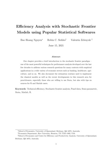
Table 3: Illustration for implementation of the Pitt and Lee (1981) model in the randomeffects framework* ********************** ** Illustration for implementation of the Pitt and Lee ( 1981 ) model **** * * * * * * * * * * * * * * * * * * * * * * * * * * * Partial Stata Codes * * * * * * * * * * * * * * * * * * * * * * * * ** *********************/* Note that output , inputs are in log forms and stored in global Statavariables y , xlist , respectively *//* Implementation using the standard Stata commands */predict ineff PL 1 , u /* Predict inefficiency , i . e . , E ( u e ) */predict eff PL 1 , te /* Predict inefficiency , i . e . , E ( exp ( - u ) e ) *//* Implementation using the commands from Belotti et al . ( 2013 ) */sfpanel y xlist , model ( pl81 )predict ineff PL 2 , u /* Predict inefficiency , i . e . , E ( u e ) */predict eff PL 2 , bc /* Predict inefficiency , i . e . , E ( exp ( - u ) e ) */vit as discussed in Pitt and Lee (1981) and Schmidt and Sickles (1984). The model thencan be estimated using the maximum likelihood estimator and the individual technicalefficiency can be obtained by employing the JLMS procedure (extended to the panel datasetting by Kumbhakar, 1987). This model is estimated in Stata using the user-writtencommand sfpanel from Belotti et al. (2013) with the option model(pl81). Alternatively,if one assumes that ui follows a truncated normal distribution, i.e., ui N (µ, σu2 ), thenthe official Stata command xtfrontier with the option ti can be utilised. A snippet ofStata codes for implementing the Pitt and Lee (1981) model is provided in Table 3.Estimation of the Schmidt and Sickles (1984) model also can be implemented in Matlaband R using the codes provided by Sickles and Zelenyuk (2019) and Sickles et al. (2020)(see the download links in footnote 14 and footnote 15).3.3Cornwell et al. (1990) ModelThe technical inefficiency estimated within the Schmidt and Sickles (1984) framework istime-invariant, which may be an unrealistic restriction in many applied settings, especiallyin a long panel. To allow for time varying inefficiency in the Schmidt and Sickles (1984)framework, one can follow the suggestion in Cornwell et al. (1990) to replace ci by, e.g.,cit , where cit is a quadratic function of time trend t with the parameters (coefficients)10
being firm-specific, specificallycit θ0i θ1i t θ2i t2 .(10)The parameters in (10) can be estimated by regressing the residual from the model (7) forproduction unit i on a constant, time, and time-squared (see more discussion in Cornwellet al., 1990). The fitted value from this model provides us with a consistent estimate (forlarge N ) of cit , denoted as ĉit . The individual technical inefficiency of production uniti at time t then can be estimated using an analogous procedure to Schmidt and Sickles(1984), specifically16ûit ĉt ĉit ,(11)whereĉt max (ĉjt ) ,j3.4t 1, . . . , T.(12)Implementation of Cornwell et al. (1990) ModelEstimation of the Cornwell et al. (1990) model can be implemented using standard Stataroutines in a set of procedures similar to those we discussed for the Schmidt and Sickles(1984) model. Alternatively, one can utilise the user-written command sfpanel fromBelotti et al. (2013) with the option model(fecss). A snippet of codes for implementingthe Cornwell et al. (1990) model using sfpanel command is provided in Table 4.Being similar to the Schmidt and Sickles (1984) model, one can estimate the Cornwellet al. (1990) model in Matlab and R using the codes provided by Sickles and Zelenyuk(2019) and Sickles et al. (2020) (see the download links in footnote 14 and footnote 15).3.5Kumbhakar (1990) and Battese and Coelli (1992) ModelsIf one is willing to impose distributional assumptions on the inefficiency component (aswell as on the random disturbance term), the maximum likelihood estimation can beutilised to estimate time-varying efficiency models. Kumbhakar (1990) and Battese andCoelli (1992) appear to be the most popular models of this type. In the Kumbhakar(1990) model, time-varying inefficiency is modelled as 1uit 1 exp at bt2τi , τi iid N 0, στ2 ,16(13)Cornwell et al. (1990) outlined estimators for a general model in which any set of regressors could bedrivers of efficiency change, if efficiency was interpreted as firm-specific heterogeneity. These regressorscould be time varying. Thus the Cornwell et al. (1990) model was the first study about which we areaware to address the issue of environmental variables influencing efficiency levels.11
Table 4: Illustration for implementation of the Cornwell et al. (1990) model* ********************** Illustration for implementation of the Cornwell et al . ( 1990 ) model *** * * * * * * * * * * * * * * * * * * * * * * * * * * * Partial Stata Codes * * * * * * * * * * * * * * * * * * * * * * * * ** *********************/* Note that output , inputs are in log forms and stored in global Statavariables y , xlist , respectively *//* Implementation using the commands from Belotti et al . ( 2013 ) */sfpanel y xlist , model ( fecss )predict ineff CSS , u /* Predict inefficiency */gen eff CSS exp ( - ineff CSS ) /* Predict efficiency */ while in Battese and Coelli (1992), time-varying inefficiency is specified asuit {exp [ η (t T )]} τi , τi iid N µ, στ2 ,(14)where a,b, and η are parameters to be estimated, and in both models, the random disturbance follows a normal distribution, i.e, vit iid N (0, σv2 ).Being similar to the Cornwell et al. (1990) model, the Kumbhakar (1990) and Batteseand Coelli (1992) models extend the Pitt and Lee (1981) model by allowing the mean ofinefficiency to vary over time, but they are more parsimonious in the sense that temporal patterns only depend or one or two parameters. The Cornwell et al. (1990) model,however, has an advantage in that it allows temporal patterns to vary across productionunits. Moreover, as discussed above, estimation of the Cornwell et al. (1990) model doesnot require parametric assumptions for inefficiency term.3.6Implementation of Kumbhakar (1990) and Battese and Coelli(1992) ModelsThe Battese and Coelli (1992) model, also known as a “time decay” model, can be estimated using Stata commands in its version 16 platform as well as by using user-writtencommands. Specifically, the estimation can be implemented by using the xtfrontiercommand with the option tvd or the command sfpanel from Belotti et al. (2013) with theoption model(bc92). The official Stata command xtfrontier cannot carry out estimation of the Kumbhakar (1990) model, which is available using the option model(kumb90)with the command sfpanel from Belotti et al. (2013). A snippet of Stata codes for12
Table 5: Illustration for implementation of the Kumbhakar (1990) and Battese and Coelli(1992) models* ********************** ******* Illustration for implementation of the Kumbhakar ( 1990 )******* ************* and Battese and Coelli ( 1992 ) models * * * * * * * * * * * * * * * ** * * ** * * * * * * * * * * * * * * * * * * * * * * * Partial Stata Codes * * * * * * * * * * * * * * * * * * * * * * * * * * ** *********************/* Note that output , inputs are in log forms and stored in global Statavariables y , xlist , respectively *//* Implementation using the standard Stata commands */xtfrontier y xlist , tvd /* the Battese and Coelli ( 1992 ) model */predict ineff BC 1 , u /* Predict inefficiency , i . e . , E ( u e ) */predict eff BC 1 , te /* Predict efficiency , i . e . , E ( exp ( - u ) e ) *//* Implementation using the commands from Belotti et al . ( 2013 ) */sfpanel y xlist , model ( bc92 ) /* the Battese and Coelli ( 1992 ) model */predict ineff BC 2 , u /* Predict inefficiency , i . e . , E ( u e ) */predict eff BC 2 , bc /* Predict efficiency , i . e . , E ( exp ( - u ) e ) */sfpanel y xlist , model ( kumb90 ) /* the Kumbhakar ( 1990 ) model */predict ineff K , u /* Predict inefficiency , i . e . , E ( u e ) */predict eff K , bc /* Predict efficiency , i . e . , E ( exp ( - u ) e ) */implementing Kumbhakar (1990) and Battese and Coelli (1992) models is provided inTable 5.The estimation of the Battese and Coelli (1992) model can be implemented in Rsoftware by using the package frontier written by Coelli and Henningsen (2020). Alternatively, R users and Matlab users can utilise the codes prepared by Sickles and Zelenyuk(2019) and Sickles et al. (2020) (see the download links in footnote 14 and footnote 15).4Recent Advances of Stochastic Panel Data ModelsThe stochastic panel data models discussed so far have a major drawback in that technical inefficiency is not distinguishable from the unobserved individual heterogeneity, andthus technical inefficiency confounds with all time-invariant unobserved individual effects.Various approaches have been proposed in the literature to mitigate this (and other) issues. Here, we will focus on a few, namely Greene (2005a,b), Chen et al. (2014), Colombi13
et al. (2014), Kumbhakar et al. (2014) and Belotti and Ilardi (2018).4.1Greene (2005a,b) ModelsGreene (2005a,b) proposed a stochastic panel data model in which unobserved individualheterogeneity separates from (transitory) technical efficiency. The model is formulated asyit ci x0it β εit ,(15)εit vit uit ,
ductivity and e ciency analysis software, e.g., Daraio et al., 2019 and Daraio et al., 2020. Besides, the chapter also complements the previous contributions of Belotti et al. (2013) and Kumbhakar et al. (2015), who focused only on stochastic frontier analysis using Stata, by providing the sources on ana