Transcription
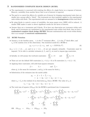
3RANDOMIZED COMPLETE BLOCK DESIGN (RCBD) The experimenter is concerned with studying the effects of a single factor on a response of interest.However, variability from another factor that is not of interest is expected. The goal is to control the effects of a variable not of interest by bringing experimental units that aresimilar into a group called a “block”. The treatments are then randomly applied to the experimentalunits within each block. The experimental units are assumed to be homogeneous within each block. By using blocks to control a source of variability, the mean square error (MSE) will be reduced. Asmaller MSE makes it easier to detect significant results for the factor of interest. Assume there are a treatments and b blocks. If we have one observation per treatment within eachblock, and if treatments are randomized to the experimental units within each block, then we have arandomized complete block design (RCBD). Because randomization only occurs within blocks,this is an example of restricted randomization.3.1RCBD Notation Assume µ is the baseline mean, τi is the ith treatment effect, βj is the j th block effect, and ij is the random error of the observation. The statistical model for a RCBD isyij µ τi βj ij and ij IIDN (0, σ 2 ).(6) µ, τi (i 1, 2, . . . , a), and βj (j 1, 2, . . . , b) are not uniquely estimable. Constraints must beimposed. To be able to calculate estimates µb, τbi , and βbj , we need to impose two constraints.aX Initially, we will assume the textbook constraints:τi 0andi 1bXβj 0.j 1 These are not the default SAS constraints (τa 0, βb 0) or R constraints (τ1 0, β1 0). Applying these constraints, will yield least-squares estimatesµb τbi and βbj where ȳi· is the mean for treatment i, and ȳ·j is the mean for block j. Substitution of the estimates into the model yields:yij µb τbi βbj eij ȳ·· (ȳi· ȳ·· ) (ȳ·j ȳ·· ) eijwhere eij b ij is the residual of an observation yij from a RCBD. The value of eij iseij yij (ȳi· ȳ·· ) (ȳ·j ȳ·· ) ȳ·· The total sum of squares (SStotal ) for the RCBD is partitioned into 3 components:a XbX(yij ȳ·· )2 i 1 j 1a XbX(ȳi· ȳ·· )2 i 1 j 1 baX bi 1ORSST otal (ȳ·j ȳ·· )2 j 1 i 1(ȳi· ȳ·· )2 ai 1aXb XaX(ȳ·b ȳ·· )2 j 1 aj 1SST rt SSBlock SSE78(yij ȳi· ȳ·j ȳ·· )2i 1 j 1bXbXa XbXa XbXi 1 j 1 a XbXi 1 j 1(yij ȳi· ȳ·j ȳ·· )2
Alternate formulas to calculate SST otal , SST rt and SSBlock .SST otal a XbX2yij i 1 j 1y··2abSST rt aXy2i·i 1SSE SST otal SST rt SSBlock3.2b wherey··2abSSBlock bXy·j2j 1a y··2aby··2is the correction factor.abCotton Fiber Breaking Strength ExperimentAn agricultural experiment considered the effects of K2 O (potash) on the breaking strength of cottonfibers. Five K2 O levels were used (36, 54, 72, 108, 144 lbs/acre). A sample of cotton was taken from eachplot, and a strength measurement was taken. The experiment was arranged in 3 blocks of 5 plots each.Block123TotalsTreatment MeansBlock MeansGrand MeanK2 O lbs/acre 5·23.55 24.16 23.23 22.54 22.35ȳ1· 7.850ȳ·1 7.630ȳ 7.723Uncorrected Sum of Squares Pai 1ȳ2· 8.053ȳ·2 7.826Pb2j 1 yijȳ3· 7.743ȳ·3 7.710Totalsy·1 38.15y·2 39.13y·3 38.55y·· 115.83ȳ4· 7.513ȳ5· 7.450 Correction factor y··2 /ab 115.832 /15 aXy2i·i 1bbXy·j2j 1a 23.552 24.162 23.232 22.542 22.3522685.5151 33 38.152 39.132 38.5524472.6815 55SST otal 895.6183 894.4393 SST rt 895.1717 894.4393 SSBlock 894.5364 894.4393 SSE 1.1790 0.7324 0.0971 Analysis of Variance (ANOVA) TableSource ofVariationSum ofSquaresd.f.MeanSquareFRatioK2 O ————Total1479p-value.0404
Test the hypotheses H0 : τ1 τ2 τ3 τ4 τ5 0 versus H1 : τi 6 0 f or some i. The test statistic is F0 4.1916. The reference distribution is F (a 1, (a 1)(b 1)) F (4, 8). The critical value is F.05 (4, 8) . The decision rule is to reject H0 if the test statistic F0 is greater than F.05 (4, 8).Is F0 F.05 (4, 8)? Is? The conclusion is toH0 and conclude thatSAS Output for the RCBD ExampleANOVA RESULTS FOR STRENGTH BY TREATMENTThe GLM ProcedureDependent Variable: strengthSourceDFSum ofSquares Mean Square F Value Pr FModel6 0.829560000.13826000Error8 0.349480000.04368500Corrected Total3.160.067714 1.17904000R-Square Coeff Var Root MSE strength Mean0.7035892.7066770.2090107.722000Source DF Type III SS Mean Square F Value Pr 00.048560001.110.3750ParameterStandardError t Value Pr t EstimateIntercept7.438000000B 0.1427807252.09 .0001k2O360.400000000B 0.170655602.340.0471k2O540.603333333B 0.170655603.540.0077k2O720.293333333B 0.170655601.720.1240k2O1080.063333333B 0000000B 0.13218926-0.610.5618block20.116000000B 0.132189260.880.4058block30.000000000B.Note: The X'X matrix has been found to be singular, and a generalized inverse was used to solve the normal equations. Terms whose estimatesare followed by the letter 'B' are not uniquely estimable.80
Fit Diagnostics for .200-1-1-2-2-0.27.47.67.88.08.27.47.6Predicted Value8.08.20.50.08.20.58.00.47.87.60.1The GLM Procedure7.20.00127.27.4 7.6 7.8 8.0RESULTS FOR STRENGTH BY TREATMENTDistribution ofANOVAstrengthQuantilePredicted ValueThe GLM 15Parameters7Error DF8MSE0.0437R-Square0.7036Adj R-Square 0.48130.28.00.0-0.27.87.6-0.407.6-0.48 -0.2400.24 0.480.0 0.4 0.8Residual0.0 0.4 0.8Proportion Less7.47.47.23654ANOVA RESULTS FOR STRENGTH BY TREATMENT7210815 k2O7.2blockDependent2 Variable: strength112strength144The GLM Procedure33blockLevel ofblockN10Observation107.85Interaction Plot for rdError t Value Pr t K2O 360.128000000.107932081.190.2697MeanStd DevK2O 540.331333330.107932083.070.015415 7.630000000.35972211K2O 720.021333330.107932080.200.848225 7.826000000.24047869K2O 108-0.208666670.10793208-1.930.089335 7.710000000.28853076K2O 70.3ANOVA RESULTS FOR-0.2STRENGTH BY TREATMENT-20.6LeverageCook's DstrengthResidual7.8Predicted Value0.2strengthstrengthDependent Variable: strength15
Critical Value of Studentized RangeANOVA RESULTS FOR STRENGTH BY TREATMENTThe GLM ProcedureTukey's Studentized Range (HSD) Test for strengthMinimum Significant Difference0.05Critical Value of Studentized Range0.2033 -0.38620.7929854 - 720.3100 -0.27960.89960.04368554 - 1080.5400 -0.04961.12960.60331.1929 ***54 - 1444.88569Minimum Significant Difference0.5896Means with the same letter are notsignificantly different.Tukey GroupingAABABABABA3.3-0.2033 -0.79290.386236 - 720.1067 -0.48290.696236 - 1080.3367 -0.25290.926236 - 1440.4000 -0.18960.989672 - 54-0.3100 -0.89960.2796N k2O72 - 36-0.1067 -0.69620.48298.05333 5472 - 1080.2300 -0.35960.819672 - 1440.2933 -0.29620.8829108 - 54-0.5400 -1.12960.0496108 - 36-0.3367 -0.92620.2529108 - 72-0.2300 -0.81960.3596108 - 1440.0633 -0.52620.65297.85007.74337.51333 363 723 108BB7.45003 144144 - 54-0.6033 -1.1929 -0.0138 ***144 - 36-0.4000 -0.98960.1896144 - 72-0.2933 -0.88290.2962144 - 108-0.0633 -0.65290.5262SAS Code for Cotton Fiber Breaking Strength RCBDDM ’LOG; CLEAR; OUT; CLEAR;’;OPTIONS NODATE NONUMBER LS 76;ODS GRAPHICS ON;ODS PRINTER PDF file ************************;*** A RANDOMIZED COMPLETE BLOCK DESIGN A in; INPUT k2O36 1 7.6236 254 1 8.1454 272 1 7.7672 2108 1 7.17108 2144 1 7.46144 20.013836 - 54MeanABSimultaneous95%ConfidenceLimits54 - 36Error Degrees of FreedomError Mean Square0.5896Comparisons significant at the 0.05 level areindicated by ***.DifferenceNote: This test controls the Type I experimentwise error rate, but it generally has a higher Type II error ratethan REGWQ.k2OBetweenComparisonMeansAlpha4.88569block strength @@; CARDS;8.0036 3 7.938.1554 3 7.877.7372 3 7.747.57108 3 7.807.68144 3 7.21PROC GLM DATA in PLOTS (ALL);CLASS k2O block;MODEL strength k2O block / SS3 SOLUTION;MEANS block;MEANS k2O / TUKEY CLDIFF LINES;ESTIMATE ’K2O 36’ K2O 4 -1 -1 -1 -1 / DIVISOR 5;ESTIMATE ’K2O 54’ K2O -1 4 -1 -1 -1 / DIVISOR 5;ESTIMATE ’K2O 72’ K2O -1 -1 4 -1 -1 / DIVISOR 5;ESTIMATE ’K2O 108’ K2O -1 -1 -1 4 -1 / DIVISOR 5;ESTIMATE ’K2O 144’ K2O -1 -1 -1 -1 4 / DIVISOR 5;TITLE ’ANOVA RESULTS FOR STRENGTH BY TREATMENT’;RUN;82
3.4Restrictions on Randomization Two common reasons for blocking:1. The experimenter has multiple sets of experimental units that are homogeneous within setsbut are heterogeneous across sets. This typically occurs when there is not a sufficient numberof homogeneous experimental units available to run a CRD leading the experimenter to formgroups of units that are as homogeneous as possible.2. The experimenter has time constraints that do not allow a CRD to be run within a continuousperiod of time that would ensure uniformity of experimental conditions. Under these circumstances, blocks take the form of a time unit (such as a day). For a RCBD, there is one restriction on randomization. Randomization is restricted to randomlyassigning the a treatments to the a experimental units within each block. In their Design of Experiments text, Anderson and McLean (A&M) introduce a random componentcalled a restriction error into the traditional RCBD model to present a more realistic picture ofthe experimental situation. This approach will be useful later when we have multiple restrictions onrandomizations (e.g., split-plot designs). Essentially, we’re saying there must be a different error structure between a completely randomizeddesign and a design that has a restriction on randomization. And, because there is a different errorstructure, there must be differences in the model and the analysis. Thus, A&M suggest that the traditional modelyij µ τi βj ij(7)should include a term indicating where the restriction on randomization occurred. That is:yijk µ τi βj δj ij(8)where µ, τi , and βj are the same in (8) as in (7), yij is the response from the ith treatment in blockj for the k th randomization, and δj is the restriction error associated with the j th block. We also assume δj N (0, σδ2 ), and each δj is completely confounded with the j th block effect.Comparison of CRD and RCBD ANOVA TablesSourceBlocksTreatmentsErrorCRD with 2 model effectstermd.f.EMSβjb 1σ 2 aφ(β) Pa2τia 1σ2 bi 1 τi /(a 1) ij(a 1)(b 1) σ 2SourceBlocksRestriction ErrorTreatmentsErrorRCBD from A&Mtermd.f.EMSβjb 1σ 2 aσδ2 aφ(β)δj(k)0σ 2 aσδ2 Pa2τia 1σ2 bi 1 τi /(a 1) ijk (a 1)(b 1) σ 2where φ(β) is a function of β1 , . . . , βb if blocks are fixed or φ(β) σβ2 if blocks are random.83
In both the fixed and random block cases, the ANOVA F -tests associated with treatment effects areidentical. You use F0 M Strt /M SE to testH0 : τ1 · · · τa 0againstH1 : not all of the τi s are equal(9) The EMS for the RCBD indicates that the correct denominator EMS for testing for a significantblock effect (either fixed or random) is the EMS for the restriction error. The problem is that this isnot estimable from the data. Under these circumstances, the test of the hypothesis involving the combination of the block effectsand the restriction error in (10) would be appropriate to test for a ‘general’ blocking effect. The statistic F M Sblocks /M SE is actually a test ofH0 : σδ2 φ(β) 0againstH1 : σδ2 φ(β) 6 0(10)Note that even if β1 β2 · · · βb 0 (fixed) or σβ2 0 (random) is true, we still have therestriction error in the EMS which prevents it from matching the error EMS σ 2 . Because of the restriction on randomization, A&M claim that there is no F test for blocks. Thatis, there is no test for H0 : σβ2 0 if blocks are random and no test for H0 : β1 β2 · · · βb ifblocks are fixed. Fortunately this is not a problem because most of the time the experimenter is only interested inwhether or not blocking had been effective in reducing the M SE for improved testing of the effectsof the treatment of interest.3.5Example of an Analysis With and Without BlocksThree different disinfecting solutions are being compared to study their effectiveness in stopping the growthof bacteria in milk containers. The analysis is done in a laboratory, and only three trials can be run onany day. Because days could represent a potential source of variability, the experimenter decides to usea randomized block design with days as blocks. Observations are taken for four days. The inside of themilk containers are covered with a certain amount of bacteria. The response is the percentage of bacteriaremaining after rinsing the container with a disinfecting solution.DaySolution1234123131652224418171394422 The data were analyzed assuming two different models. The first model does not include blocks.The second model includes blocks. The SAS analysis for both models is on the next page. Here areimportant results:84
Without blocksWith blocksR2M SEp-value Note that we would fail to reject H0 if blocks were not in the model because there is large variabilityacross blocks (M Sday 368.97). If the SSday 1106.92 and dfday 3 is pooled with the the SSE 41.83 and dfE 6 in the modelwith days (blocks), then it forms the SSE 1158.75 and dfE 9 for the model without days (blocks).SAS Code for RCBD Analyses With and Without BlocksDM ’LOG;CLEAR;OUT;CLEAR’;ODS GRAPHICS ON;* ODS PRINTER PDF file ’C:\COURSES\ST541\RCBD2.PDF’;OPTIONS NODATE NONUMBER LS 76 PS ** RCBD ANALYSES WITH AND WITHOUT BLOCKS DATA IN;DO solution 1 TO 3;DO day 1 TO 4;INPUT growth @@; OUTPUT;END; END;LINES;13 22 18 3916 24 17 445 4 1 ********;*** RUN AN ANOVA WITH SOLUTION ONLY, NO DAY BLOCKS *********;PROC GLM DATA IN;CLASS solution;MODEL growth solution / ss3;TITLE ’RCBD WITHOUT DAYS (BLOCKS) IN THE ;*** RUN AN ANOVA WITH DAYS AS BLOCKS ***;*****************************************;PROC GLM DATA IN;CLASS day solution;MODEL growth solution day / ss3;TITLE ’RCBD WITH DAYS (BLOCKS) IN THE MODEL’;RUN;85
EXAMPLE 9: RCBD WITH DAYS AS BLOCKSThe GLM ProcedureDependent Variable: growthInteraction Plot for growth40growth3020100EXAMPLE1 9: RCBD IGNORINGDAYSAS BLOCKS234day12solutionTheGLM Procedure3RCBD Without Days as BlocksDependent Variable: growthSum ofSquares Mean Square F Value Pr FSourceDFModel2703.500000351.750000Error9 1158.750000128.750000Corrected Total2.730.118211 1862.250000R-Square Coeff Var Root MSE growth Mean0.377769Source60.5163011.3468118.75000DF Type III SS Mean Square F Value Pr FEXAMPLE 9: RCBD WITH DAYS AS BLOCKSsolutiongrowth30SourceDF0.1182Sum ofSquares Mean Square F Value Pr FModel5 1810.416667Error6Corrected Total362.08333351.83333341.910.00018.63888911 1862.250000R-Square Coeff Var Root MSE growth Mean0.972166Source15.675732.93919918.75000DF Type III SS Mean Square F Value Pr Fsolution2703.500000351.75000040.720.0003day3 1106.916667368.97222242.710.00020Interaction Plot for growth1402.73F2.73Prob F 0.11822010351.7500000The GLM ProcedureDistribution of growthRCBD Without Days as BlocksDependent Variable: growth402 703.5000000286solution3
3.6Type I vs Type III Analyses Without the /ss3 option in the MODEL statement, SAS will contain two ANOVA tables: ANOVAfor Type I sum of squares and ANOVA for Type III sum of squares. If there are no missing observations, the Type I and Type III analyses are identical. If there are missing observations, the Type I and Type III analyses are different. To see how theydiffer we will first look at the Type I analysis.3.6.1Type I Analysis The Type I analysis is based on sequentially fitting the data to the model one factor at a time. It isoften referred to as the sequential sum of squares method. For the RCBD there are two possibilities that I will refer to as– Version 1 (V1) when fitting treatments before blocks.– Version 2 (V2) when fitting blocks before treatments. Let RSSi be the error sum of squares (SSE ) after fitting the model in the ith step. The steps for determining the ANOVA SS for V1 are:1. Fit yij µ ij and obtain RSS1 SStotal .2. Fit yij µ τi ij and obtain RSS2 SSE for the model with treatments only.3. Fit yij µ τi βj ij and obtain RSS3 SSE for the model with treatments and blocks. The steps for determining the ANOVA SS for V2 are:1. Fit yij µ ij and obtain RSS1 SStotal .20 . Fit yij µ βj ij and obtain RSS2 SSE for the model with blocks only.3. Fit yij µ τi βj ij and obtain RSS3 SSE for the model with blocks and treatments. The ANOVA sum of squares for V1 and V2 are summarized in the following table:StepV1 SourceFitdf1233TotalTreatmentBlocksErrorµτiβj ijN 1a 1b 1N a b 1StepV2 SourceFitdf12033TotalBlocksTreatmentErrorµβjτi ijN 1b 1a 1N a b 187Type I SS for V1RSS1R(τ µ)R(β τ, µ)RSS3 RSS1 RSS2 RSS2 RSS3Type I SS for V2RSS1R(β µ)R(τ β, µ)RSS3 RSS1 RSS2 RSS2 RSS3
In V1, the quantity R(τ µ) is called the reduction in SS due to τ adjusted for µ and R(β τ, µ)is called the reduction in SS for β adjusted for τ and µ. In V2, the quantity R(β µ) is called the reduction in SS due to β adjusted for µ and R(τ β, µ)is called the reduction in SS for τ adjusted for β and µ.3.6.2Type III Analysis The Type III analysis is referred to as the marginal means or the Yates weighted squares ofmeans analysis. For a RCBD, the Type III SStrt and SSblocks are computed using the following procedure:1. Fit the model with treatments only: yij µ τi ij . Then RSS2 SSE for this model.2. Fit the model with blocks only: yij µ βj ij . Then RSS2 SSE for this model.3. Fit the model yij µ τi βj ij . Then RSS3 SSE and RSS1 SStotal for the modelwith both treatments and blocks.Step1231SourceFitdfType III SSTotalTreatmentBlocksErrorµτiβj ijN 1a 1b 1N a b 1RSS1R(τ β, µ) RSS2 RSS3R(β τ, µ) RSS2 RSS3RSS3 If any yij values are missing, then SStrt SSblocks SSE 6 SStotal for a Type III analysis.3.6.3RCBD Analysis with a Missing ObservationSee the example in Section 3.5 for the description of the experiment. Suppose y23 was missing from theRCBD. The RCBD data table is:DaySolution1234123131652224418.1394422 Let us examine the Type I and Type III sums of squares. The next page contains the SAS output. The top of the next page contains the Type I (V1) sum of squares and the bottom of the page containsthe Type I (V2) sum of squares. Note the difference in sums of squares, mean squares, F-statistics,and p-values for the Type I analyses. The reason for the difference between the V1 and V2 Type I sum of squares is that a Type I analysisis sequential so the order in which terms enter the model is important. The Type III analysis is the same for both analyses Type III sums of squares are not calculatedsequentially. That is, the order in which terms enter the model is not important. The following page contains the two analyses with only one effect in each model. I included theseanalyses so you can see how RSS2 and RSS2 are calculated.88
ANOVA RESULTS (SOLUTION THEN DAY)The GLM ProcedureANOVA RESULTS: (MODEL WITH SOLUTION THEN DAY)Variable: growthSourceDFSum ofSquares Mean Square F Value Pr FModel5 1811.575758Error5Corrected Total47.333333362.31515238.270.00059.46666710 1858.909091R-Square Coeff Var Root MSE growth Mean0.974537SourceDF16.271513.07679518.90909Type I SS Mean Square F Value Pr Fsolution2790.909091395.45454541.770.0008day3 1020.666667340.22222235.940.0008SourceDF Type III SS Mean Square F Value Pr Fsolution2670.500000335.25000035.410.0011day3 1020.666667340.22222235.940.0008ANOVA RESULTS (DAY THEN SOLUTION)The GLM ProcedureANOVA RESULTS: (MODEL WITH DAY THEN SOLUTION)Variable: growthSourceDFSum ofSquares Mean Square F Value Pr FModel5 1811.575758Error5Corrected Total47.333333362.31515238.270.00059.46666710 1858.909091R-Square Coeff Var Root MSE growth Mean0.974537SourceDF16.271513.07679518.90909Type I SS Mean Square F Value Pr Fday3 035.410.0011Source670.500000DF Type III SS Mean Square F Value Pr Fday3 035.410.0011670.500000So where did RSS2 and RSS2 come from?89
ANOVA RESULTS (SOLUTION ONLY)The GLMRSS2 is the SSE for themodelProcedurewith only treatments and no blocks.ANOVA RESULTS FOR THE MODEL WITH SOLUTION (TREATMENTS) ONLYVariable: growthDFModel2790.909091395.454545Error8 1068.000000133.500000Corrected Total2.960.109010 1858.909091R-Square Coeff Var Root MSE growth 11.5542218.90909Type I SS Mean Square F Value Pr F2 790.9090909395.45454552.960.1090DF Type III SS Mean Square F Value Pr F2 790.9090909395.45454552.96ANOVA RESULTS (DAY ONLY)0.1090Distribution of growthProcedurethe GLMmodelwith only blocks and no treatments.RSS2 is the SSE for TheVariable:growthSum ofSquares Mean Square F Value Pr FSource40F2.96Prob F0.1090ANOVA RESULTS FOR THE MODEL WITH DAYS (BLOCKS) ONLYgrowthSource30DFSum ofSquares Mean Square F Value Pr FModel3 1141.075758380.358586Error7102.547619Corrected Total717.8333333.710.069610 1858.90909120R-Square Coeff Var Root MSE growth Mean0.61384253.5540310.1265818.9090910Source DFdayType I SS Mean Square F Value Pr F3 1141.075758380.3585863.710.069601SourceDF Type III SS Mean 2Square F Value Pr Fsolutionday3 1141.075758380.3585863.71 0.06963All of these calculationsDistributionare done ofautomaticallyin the RCBD analyses for the two modelsgrowthon the3.71previous page.FF3.71Prob F 0.069640Prob F 0.069690
Type I SS (V1) SummaryRSS1 1858.91R(µ) RSS1RSS2 1068.00R(τ µ) RSS1 RSS2RSS3 47.33R(β τ, µ) RSS2 RSS3 1858.91 790.91 1020.67Type I SS (V2) SummaryRSS1 1858.91R(µ) RSS1 R(β µ) RSS1 RSS2 RSS2 717.83RSS3 47.33R(τ β, µ) RSS2 RSS3 1858.91 1141.08 670.50Type III SS SummaryRSS1 1858.91R(µ) RSS1RSS3 47.33RSS2 717.83R(β τ, µ) RSS2 RSS1RSS2 1068.00R(τ β, µ) RSS2 RSS1DM ’LOG; CLEAR; OUT; CLEAR;’;ODS GRAPHICS ON;ODS PRINTER PDF file ’C:\COURSES\ST541\RCBDMISS.PDF’;OPTIONS NODATE ** RCBD WITH A MISSING OBSERVATION ***;***************************************;DATA IN;DO solution 1 TO 3;DO day 1 TO 4;INPUT growth @@; OUTPUT;END; END;CARDS;13 22 18 3916 24 . 445 4 1 ****;*** RUN AN ANOVA WITH SOLUTION APPEARING FIRST *****;PROC GLM DATA IN;CLASS solution day;MODEL growth solution day;TITLE ’ANOVA RESULTS (SOLUTION THEN ****;*** RUN AN ANOVA WITH DAY APPEARING FIRST ;PROC GLM DATA IN;CLASS day solution;MODEL growth day solution;TITLE ’ANOVA RESULTS (DAY THEN ***;*** RUN AN ANOVA WITH SOLUTION ONLY ***;****************************************;PROC GLM DATA IN;CLASS solution;MODEL growth solution;TITLE ’ANOVA RESULTS (SOLUTION ONLY)’;***********************************;*** RUN AN ANOVA WITH DAY ONLY ***;***********************************;PROC GLM DATA IN;CLASS day;MODEL growth day;TITLE ’ANOVA RESULTS (DAY ONLY)’;RUN;91 1858.91 1020.67 670.50
R code for RCBD with missing value# ANOVA for RCBD with missing observationstrength - c(13,22,18,39,16,24,NA,44,5,4,1,22)solution - c(1,1,1,1,2,2,2,2,3,3,3,3)day - c(1,2,3,4,1,2,3,4,1,2,3,4)f1 - aov(strength factor(day) factor(solution))summary (f1)f2 - lm(strength factor(day) factor(solution))summary(f2)R output for RCBD with missing value summary (f1)Df Sum Sq Mean Sq F valuePr( F)factor(day)3 1141.1380.440.18 0.000636 ***factor(solution) 2 670.5335.235.41 0.001116 **Residuals547.39.5--Signif. codes: 0 ‘***’ 0.001 ‘**’ 0.01 ‘*’ 0.05 ‘.’ 0.1 ‘ ’ 11 observation deleted due to missingness summary(f2)Coefficients:Estimate Std. Error t value Pr( t )(Intercept)15.3332.2066.952 0.000946 ***factor(day)25.3332.5122.123 0.087176 .factor(day)31.6672.9010.575 0.590479factor(day)423.6672.5129.421 0.000227 ***factor(solution)23.0002.4321.233 0.272264factor(solution)3 -15.0002.176 -6.895 0.000983 ***--Signif. codes: 0 ‘***’ 0.001 ‘**’ 0.01 ‘*’ 0.05 ‘.’ 0.1 ‘ ’ 1Residual standard error: 3.077 on 5 degrees of freedom(1 observation deleted due to missingness)Multiple R-squared: 0.9745,Adjusted R-squared: 0.9491F-statistic: 38.27 on 5 and 5 DF,p-value: 0.000546892
3.6.4Type I vs Type III Hypotheses Because of differences between Type I and Type III SS, there will be differences in the hypothesesassociated with the F -tests (assuming the restriction on randomization is ignored). Let µij µ τi βj be the ith treatment, j th block mean.Hypotheses for Type III and Type I (V2) Sum of SquaresH0 : µ1· µ2· · · · µa·H1 : µi· 6 µi · for some i 6 i bXand µi· µij /b.j 1Hypotheses for Type I (V1) Sum of SquaresH0 :bbb1 X1 X1 Xn1j µ1j n2j µ2j · · · naj µajn1·n2·na·j 1H1 :j 1j 1bb1 X1 Xnij µij 6 ni j µi j for some i 6 i .ni·ni ·j 1j 1where ni· the number of nonmissing yij values for the ith treatment, and nij 1 if yij is not missingand nij 0 if yij is missing. The Type III hypotheses are comparing the treamtment means average across the blocks (and arethe ones I want to test.) Therefore I recommend using the p-values from a Type III analysis. If there are no missing yij values, the Type I and Type III hypotheses are the same.3.7RCBD Normal Equations For model yij µ τi βj ij , the error is ij yij µ τi βj Substituting in estimates produces the residual b ij eij yij µb τbi βbj . Goal: Find µb, τbi , and βbj that minimize L:L a XbXi 1 j 1b ij2 a XbX(yij µb τbi βbj )2i 1 j 1 Solution: Solve the normal equations L µb L bτi L βbja XbX 2(yij µb τbi βbj ) 0i 1 j 1bX 2(yij µb τbi βbj ) 0 2j 1aX(yij µb τbi βbj ) 0i 193for i 1, 2, . . . , afor j 1, 2, . . . , b
After distributing the sum and then simplifying, we get:(i)y·· abbµ baXτbi abXi 1(ii)yi· bbµ b τbi βbjj 1bXβbjfor i 1, 2, . . . , aτbi aβbjfor j 1, 2, . . . , bj 1(iii)y·j abµ aXi 1 For (i), (ii), and (iii), there is a total of 1 a b equations. If you sum the a equations in (ii), youget (i). If you sum the b equations in (iii), you also get (i). Thus, the rank is a b 1 which impliesthat µ and each τi and βj are not uniquely estimable. To get estimates of µ and each τi and βj , weabXXmust impose 2 constraints. We will useτi 0 andβj 0.i 1j 1 Substitution of these constraints into (i), (ii), and (iii) yields(1) abbµ y··(2) bbµ bbτi yi· Then, from (1), we haveµb (3) abµ aβbj y·jy·· ab Substitution of µb y ·· in (2) yields:by ·· bbτi yi· y ·· τbi y i· τbi y ·· βbj y ·j βbj Substitution of µb y ·· in (3) yields:ay ·· aβbj y·j3.8Matrix Forms for the RCBDExample: The goal is to determine whether or not four different tips produce different readings on ahardness testing machine. The machine operates by pressing the tip into a metal test coupon, and fromthe depth of the resulting depression, the hardness of the coupon can be determined. The experimenterdecides to obtain four observations for each tip. Four randomly selected coupons (blocks) were used andeach tip (treatment) was tested on each coupon. The data represent deviations from a desired depth in0.1 mm units:Type of TipType of Coupon12341234 2 115 1 234 3 102215794
Model: yij µ τi βj ij for i 1, 2, 3, 4 and j 1, 2, 3, 4 ij N (0, σ 2 )βj N (0, σβ2 )P4P4 Assume (i)i 1 τi 0 and (ii)j 1 βj 0. If we estimate [ µ, τ1 , τ2 , τ3 , β1 , β2 , β3 ] , we canthen estimate τ4 τ1 τ2 τ3 from (i)andβ4 β1 β2 β3 from (ii). X X 0X 010-1010-1010-1001-1001-1001-1001-1 y 1 16 20-12-11-17-22-21-9 1 (X 0 X) 1 X 0 y 16 1 16 (X 0 X) 15/4-2/4-1/4-7/4-9/4-8/44/4Thus, τb4 bτ1 τb2 τb3 10/4 and95y ··y 1· y ··y 2· y ··y 3· y ··y ·1 y ··y ·2 y ··y ·3 y ··-2-115-1-234-3-1022157 1 0 0 0 0 0 00 3 -1 -1 0 0 0 0 -1 3 -1 0 0 0 0 -1 -1 3 0 0 0 0 0 0 0 3 -1 -1 0 0 0 0 -1 3 -1 0 0 0 0 -1 -1 -1β20484000 0000484β10844000 X 0y 0000844τ320-36 11 1712 - 33 1712 11 -51-66 21 922 - 63 922 21 -27 µbτb1τb2τb3bβ1βb2βb3 βb4 βb1 βb2 βb3 13/4
Alternate Approach: Keeping a b 1 Columnsµ X 0XX 0100010001000101 y 1 16 3 1 1 1 1 1 1 1 1 140000000 104000000 100400000 100040000 100004000 100000400 100000040 1110411151111411115111411111511 2034 215 4 3918 0 1 0(X X) X y 0Xy 411111151000000001111000010τ4(X 0 X) 1965/4 2/4 1/4 7/410/4 9/4 8/44/413/4 2 115 1 234 3 102215700
block, and if treatments are randomized to the experimental units within each block, then we have a randomized complete block design (RCBD). Because randomization only occurs within blocks, this is an example of restricted randomization. 3.1 RCBD Notation Assume is the baseline mean,
