Transcription
Class Notes, 31415 RF-Communication CircuitsChapter IIRF-CIRCUITSJens VidkjærNB230
ii
ContentsII RF-Circuits, Concepts and Methods . . . . . . . . . . . . . . . . . . . . . . . . . . . . . . . .II-1 Parallel Resonance Circuits . . . . . . . . . . . . . . . . . . . . . . . . . . . . .Frequency Response . . . . . . . . . . . . . . . . . . . . . . . . . . . . . . . .Poles and Zeros . . . . . . . . . . . . . . . . . . . . . . . . . . . . . . . . . . . .Transient Response . . . . . . . . . . . . . . . . . . . . . . . . . . . . . . . . .II-2 Series Resonance Circuit Summary . . . . . . . . . . . . . . . . . . . . . . . .II-3 Narrowband Approximations . . . . . . . . . . . . . . . . . . . . . . . . . . . .II-4 Series-to-Parallel Conversions . . . . . . . . . . . . . . . . . . . . . . . . . . . .Example II-4-1 ( impedance matching ) . . . . . . . . . . . . .Conversions in Narrowband Applications . . . . . . . . . . . . . . . . . .Conversions in Broadband Modeling . . . . . . . . . . . . . . . . . . . . .Example II-4-2 ( spiral inductor ) . . . . . . . . . . . . . . . . .II-5 Tuned Amplifiers . . . . . . . . . . . . . . . . . . . . . . . . . . . . . . . . . . . . .Synchronously Tuned Amplifiers . . . . . . . . . . . . . . . . . . . . . . . .Example II-5-1 ( synchronous tuning ) . . . . . . . . . . . . . .Butterworth Stagger Tuned Amplifiers . . . . . . . . . . . . . . . . . . .Example II-5-2 ( Butterworth amplifier ) . . . . . . . . . . . .II-6 Transformers and Transformerlike Couplings . . . . . . . . . . . . . . . . . .Review of Mutual Inductances . . . . . . . . . . . . . . . . . . . . . . . . .Equivalent Circuits for Two Coupled Inductors . . . . . . . . . . . . . .RF-Transformers . . . . . . . . . . . . . . . . . . . . . . . . . . . . . . . . . . .Example II-6-1 ( practical RF transformers ) . . . . . . . . .Tuned Transformers . . . . . . . . . . . . . . . . . . . . . . . . . . . . . . . . .Example II-6-2 ( transformer-coupled tuned amplifier ) . .Autotransformers . . . . . . . . . . . . . . . . . . . . . . . . . . . . . . . . . . .Example II-6-3 ( autotransformers in a tuned amplifier ) .Transformerlike Couplings . . . . . . . . . . . . . . . . . . . . . . . . . . . .Example II-6-4 ( uncoupled reactance transformers intuned amplifiers ) . . . . . . . . . . . . . . . . . . . . . .Three-Winding Transformers . . . . . . . . . . . . . . . . . . . . . . . . . .Transformer Hybrids . . . . . . . . . . . . . . . . . . . . . . . . . . . . . . . .Example II-6-5 ( diode-ring mixer preliminaries ) . . . . . .II-7 Double-Tuned Circuits and Amplifiers . . . . . . . . . . . . . . . . . . . . . . .Coupling between Identical Resonance Circuits . . . . . . . . . . . . . .Example II-7-1 ( Foster-Seely FM detector ) . . . . . . . . .Example II-7-2 ( quadrature FM detector ) . . . . . . . . . . .Double-Tuned Amplifier Stages . . . . . . . . . . . . . . . . . . . . . . . .Asymptotic Behavior . . . . . . . . . . . . . . . . . . . . . . . . . . . . . . . .II-8 Impedance Matching . . . . . . . . . . . . . . . . . . . . . . . . . . . . . . . . . . 53555758616263.64677278808185889498101
Lumped Element Impedance Matching using Smith Charts . .Example II-8-1 ( double and standard Smith charts )Example II-8-2 ( bandwidth estimations ) . . . . . . . .APPENDIX II-A, Power Calculation and Power Matching . . . . . . . .APPENDIX II-B Signal Flow Graphs . . . . . . . . . . . . . . . . . . . . . .Elementary Signal Flow Graphs . . . . . . . . . . . . . . . . . . . .Mason’s Direct Rule . . . . . . . . . . . . . . . . . . . . . . . . . . . .Problems . . . . . . . . . . . . . . . . . . . . . . . . . . . . . . . . . . . . . . . . . .References and Further Reading . . . . . . . . . . . . . . . . . . . . . . . . . .101104108113117117121125131Index . . . . . . . . . . . . . . . . . . . . . . . . . . . . . . . . . . . . . . . . . . . . . . . . . . . . . . . . . 133ivJ.Vidkjær
1II RF-Circuits, Concepts and MethodsIn RF-communication system, control of frequency bands and impedance matchingconditions between functional blocks or amplifier stages are problems that constantly face acircuit designer. The tasks are so frequent that many analytical techniques and approximationmethods especially suited for high-frequency circuits have evolved and strongly influenced thejargon of RF engineering. Below we shall introduce the most important basic concepts andmethods that are required to- understand data sheets and literature,- make simpler design decisions or calculations, and- prepare and interpret simulation data.The selection of topics and examples have furthermore been conducted to suit the needs inthe following chapters, which are still in preparation.Scanning contents, the chapter starts summarizing basic properties of resonancecircuits. Although significant by themselves, the importance of acquiring familiarity with idealresonance circuits is the fact, that any narrowbanded resonance circuit may be approximatedby the ideal ones around resonance frequencies. This property reduces significantly the effortsthat are required to understand and explore operations of tuned bandpass circuits, which arefrequently used in RF-communication systems. Foundations of the simplifications are dealtwith in sections concerning narrowband approximations and series-to-parallel transformations.The tuned amplifiers are introduced in ideal form concentrating on simple frequency characteristics. Coupling techniques using transformers and coupled resonance circuits are still highlyuseful methods in RF-designs, so they are considered in some details here. Finally, the verygeneral method of constructing lumped element matching networks using a Smith chart isexemplified.Power matching is fundamental for designing and understanding many RF circuits.Although this concept is mandatory in basic circuit theory curriculums, it is repeated forconvenience in an appendix. Also the method of illustrating and solving network equationsby the signal flow graph method is summarized in an appendix.J.Vidkjær
2II-1 Parallel Resonance Circuits(1)Fig.1 Parallel resonance circuitA basic parallel resonance circuit is shown in Fig.1. Besides component values thecombinations, which are summarized by Eq.(1), are frequently used. The resonance frequencyis the frequency where the capacitive and the inductive susceptances are equal in magnitudeas indicated in Fig.2a. When an external steady state sinusoidal voltage-source of frequencyω0 is applied to the resonance circuit, the two opposite currents through the capacitor and theinductor balance each other, and only the resistor current flows through the terminal. Thissituation is sketched in Fig.2b, which also shows how the quality factor Q indicates themagnitude ratio of the internal reactive currents over the resistive terminal current at resonance.Fig.2Parallel resonance. (a) Susceptance composition as function of frequency. (b)Current and voltage phasors at the resonance frequency ω0.Another view upon resonance and the quality factor concerns the energy in the circuitunder steady state conditions. At instants where the two phasors iC and iL are perpendicularto the real axis, no currents flow into the capacitor or inductor, but the capacitor holdmaximum energy(2)J.Vidkjær
II-1 Parallel Resonance Circuits3The first equation is the usual electrostatic energy expression. The second takes into accountthat rms values - indicated by small letters - are conventionally used when dealing with steadystate linear circuits. A quarter of a period later the current phasors project in full onto the realaxis while the voltage is zero. The capacitor holds no energy, but the inductor energy peakswith the same maximum that formerly was held in the capacitor,(3)Thus, a constant amount of energy laps between the capacitor and the inductor at resonance,and the quality factor may be expressed(4)where the loss is calculated as the resistor power times the resonance period T0 2π/ω0. Thisinterpretation of resonance is often useful in the construction of lumped circuit equivalents forthe variety of electromagnetic and mechanical resonators that are used in RF-circuits.Frequency ResponseExpressed through circuit element values, the impedance function for the parallelcircuit in Fig.1 is(5)Introducing ω0 and Q from Eq.(1), the impedance expressed as a function of frequency s jωbecomes(6)The frequency dependency of the impedance is kept in the quantity β(ω), which is zero at theresonance frequency ω0. Here the denominator of Eq.(6) gets its smallest size and theimpedance has maximum Rp, the parallel resistance. The magnitude and phase of Zp(jω) are(7)The two functions are shown in Fig.3(a) while Fig.3(b) shows the corresponding admittancecharacteristics,J.Vidkjær
4Fig.3RF-Circuits, Concepts and MethodsImpedance (a) and admittance (b) magnitudes and phases of the parallel resonancecircuit in Fig.1. The curves are symmetric around ωo due to the logarithmic frequency scales.(8)Upper and lower bounds of the 3dB bandwidth intervals W3dB, which are indicatedin Fig.3 , correspond to a denominator size equal to 2 in Eq.(7). The bounds are foundsetting the imaginary part of the denominator equal in magnitude to the real part, i.e.(9)Both negative and positive frequencies are contained in the conditions. We call the largestvalued solutions, where the two terms in ωb have equal signs, the upper bounds ωbu. Thelower bounds ωbl are obtained with terms of opposite signs. Fig.4 summarizes how thedifferent solutions are formed. By definition, the 3dB bandwidth is taken to be the distancebetween positive or zero-valued 3dB frequency bounds, and we get the result that wasincorporated in Fig.3,(10)It follows from the solutions in Eq.(9) that the resonance frequency ω0 is not centered betweenthe 3dB bounds but is the geometrical mean of the bounds,J.Vidkjær
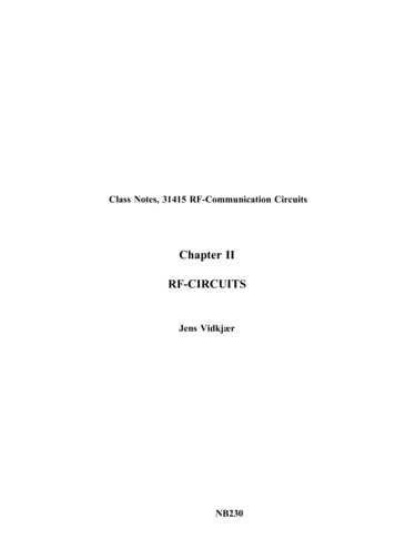
II-1 Parallel Resonance CircuitsFig.45Upper and lower 3dB bound positions from Eq.(9) . Note, in linear frequency scalethe 3dB bands are not symmetric around the resonances at ω0 unless Q .(11)(12)so in logarithmic frequency scale the upper and lower 3dB frequency bounds are symmetricwith respect to logω0. However, any other pair of frequencies, ωu,ωl that has the resonancefrequency as geometrical mean maps symmetrically around logω0. Since both frequenciesprovide the same absolute β , i.e.(13)the impedance or admittance magnitude characteristics of the types in Fig.3 have evensymmetry with respect to the resonance frequency in a logarithmic frequency scale. Correspondingly, the phase characteristics show odd symmetry because tan-1(-Qβ) -tan-1(Qβ). Atthe 3dB boundaries where Qβ 1, the phase angles of impedance Zp become ¼π. Fig.5shows plots of the impedance function with various Q-factors. The normalization in magnitudecorresponds to keeping the inductor and capacitor fixed while letting the parallel resistancefollows Q according to Eq.(1). The asymptotic behavior of the impedance approximating theinductor reactance below and the capacitor reactance above resonance respectively are readilyobserved. Calculating magnitudes, it may suffice to use the inductor or capacitor alone atfrequencies that differ more than a factor of three from resonance.Summarizing the frequency characteristics, we have seen that the greater Q, thesmaller bandwidth and in turn, the steeper phase characteristics around the resonance frequency ω0. Moreover, the frequency characteristics were symmetric in logarithmic frequency scale.Phase steepness is an important property when a resonance circuit is employed in an oscillatorand we shall return to this question later. Also, the symmetry property will be reconsidered.Important classes of signal handling expect linear symmetry that may be approached with highJ.Vidkjær
6Fig.5RF-Circuits, Concepts and MethodsNormalized magnitudes and phases in the impedance of parallel tuned circuits withvarying Q-factors.Q circuits too.1 For obvious reasons such circuits are also called narrowbanded.Poles and ZerosPole and zero positions are useful for investigating responses of frequency selectivenetworks that include parallel tuned circuits. Using parameters from Eq.(1), the impedance Zpof Eq.(5) is rewritten,(14)Solving for the s-values, which set the numerator and the denominator equal to zero respectively, gives the zero and the poles of the impedance function. Once poles and zeros areknown, the impedance may be cast in the form that suits the analysis of composite networks,(15)1)See section VI-1 on frequency stability in oscillators and section I-4 on transmissionof narrowband signals.J.Vidkjær
II-1 Parallel Resonance Circuits7While there is a tradition of using Q for characterizing frequency responses ofresonant RF circuits, the conceptually equivalent damping ratio ζ is often seen in pole-zeroand especially transient response calculations, where it leads to more compact expressions. Weproceed here with both forms and get,(16)Up to this point no attention was given to actual parameter values. The last result requires adistinction between circuits having ζ 1 and ζ 1 ( Q ½ and Q ½ ). In first case the squareroots of Eq.(16) are real and the poles are on the real axis. In second case the poles movefrom the real axis and make a complex conjugated pair. To emphasize this property we changethe last part of Eq.(16) to read(17)Fig.6Position of poles s1, s2, and the zero s0 in the impedanceZp(s) of the parallel resonance circuit with ζ 1 or Q ½.The square roots in (a) are real valued if the poles are complex. The approximations in thefollowing lines apply to lightly damped circuits with higher and higher Q s, where theJ.Vidkjær
8RF-Circuits, Concepts and Methodsexpressions in Eq.(17)(b) are based on the estimate(18)Fig.6 sketches the geometry of complex pole and zero positions. Starting from damping ζ 1( Q ½) the poles are by Eq.(17)(a) constrained to move along a circle of radius ω0 from thereal towards the imaginary axis with declining damping or growing Q. Once the poles andzeros are known, the frequency characteristics of Zp may be calculated from geometricalconsiderations as sketched in Fig.7 and Eqs.(19) to (21).(19)(20)(21)Fig.7Calculation of Zp(ω) from polesand zerosTransient ResponseFig.8Charging of capacitor C to voltage VC0 QC0/C.The projection of the poles on the imaginary axis determines the oscillatory modesin the transient responses of the circuit. To see this, we consider the decay of circuit energywhen the circuit is left alone once the capacitor has been charged to a voltage of VC0 with theinductor current initialized to zero. The initial charging of the capacitor is equivalent toforcing a pulse current of strength(22)J.Vidkjær
II-1 Parallel Resonance Circuits9through the circuit as indicated by Fig.8.2 The corresponding transient voltage decay Vdcy(t)is the impulse response of the impedance function, which is given by its inverse Laplacetransform, i.e.(23)The last rewriting prepares for use of standard Laplace transform tables, from which we get(24)where the angular frequency is recognized as the size of the imaginary pole component if ζ 1.Introducing the auxiliary phases and the identities(25)(26)(27)the time domain responses may be condensed to read(28)2)J.VidkjærNote, the delta function δ(t) has dimension [sec-1] to comply with the requirement
10Fig.9RF-Circuits, Concepts and MethodsTransients from Eq.(28). Examples in (a) are heavily damped and (b) is lightlydamped. Time scales are in units of the resonance period T0 2π/ω0.Fig.9 shows examples of the responses with different dampings. The case ζ 1, where the twopoles coincide on the real axis, sets the border between aperiodic and oscillatory solutions. Inthe latter case, the leading exponential factor shapes the envelope to the solution(29)The corresponding time constant,(30)is sometimes called the logarithmic decrement of the circuit. Observe that the result is inagreement with the previous equivalent baseband considerations in example I-4-2. In practicalterms we notice that the significant number of cycles through the decay approximates Q if Q 5 so ζ 0.1 and cosφ1 1. It follows from the fact that at t QT0, the exponential has fallenfrom one to(31)so more than 99.8% of the initial energy is lost in the resistor at that instant.J.Vidkjær
11II-2 Series Resonance Circuit Summary(32)Fig.10 Series resonance circuitA series resonance circuit is connected as shown by Fig.10 and Eq.(32) summarizesits common parameter combinations. The circuit admittance and impedance are,(33)Compared to the parallel circuit impedance and admittance in Eq.(5) it is seen, that thenumerator and denominator are similar in structure with respect to s, but the coefficients aredifferent. Connected to a source, the two types of resonance circuits behave in duality. Thismeans that the reader could kindly be asked to repeat the preceding section exchanging terms,voltage and current, parallel and series, impedance and admittance, inductance and capacitance, resistance and conductance, and then we were done. To avoid confusion in futurereferences, however, the main concept of the series resonance is summarized below in its ownterms, but without detailed derivations.Fig.11Series resonance. (a) Reactance composition as function of frequency. (b) Voltageand current phasors at the resonance frequency ω0.At resonance in a series circuit the voltages across the inductive and the capacitivereactances are equal in magnitudes but opposed in phases. With the same current flowingthrough all components the requirement is that the two reactances balance each other at theJ.Vidkjær
12RF-Circuits, Concepts and Methodsresonance frequency as indicated by Fig.11(a). The phasor diagram in Fig.11(b) shows thatthe quality factor now represents the ratio of the reactance voltage magnitudes over the voltagevR across the series resistor Rs. At resonance this voltage equals the terminal voltage v. Withone terminal grounded, the potential at the interconnection between the inductor and thecapacitor becomes Q times as high as the potential at the driving terminal. This fact maysignificantly influence the practical realization of high Q series circuits.Like the parallel circuit in steady state resonance, a constant amount of energy isexchanged between the capacitor and the inductor in the series circuit. In terms of energythere are no differences between the two types of resonance circuits regarding the qualityfactor, but the loss calculation must now be detailed as a series loss,(34)Using the resonance frequency and the quality factor from Eq.(32) the impedance ofthe series circuit is expressed(35)The frequency is again accounted for through β(ω), so the impedance and admittance functions become symmetric in logarithmic frequency scales as showed in Fig.12.Fig.12Impedance (a) and admittance (b) magnitudes and phases of the series resonancecircuit in Fig.10. The curves are symmetric around ωo due to the logarithmic frequency scales.Impedance and admittance magnitudes and phases in Fig.12(a) and (b) are given byJ.Vidkjær
II-2 Series Resonance Circuit SummaryFig.1313Normalized magnitude and phases for the impedance of series resonance circuitswith varying Q-factors.(36)(37)The equations are equivalent to Eqs.(8) and (7), so all results concerning bandwidth andsymmetry of bounds and characteristics may directly be overtaken from the forgoing section.Fig.13 holds impedance characteristics with different Q-factors and shows the asymptotes setby the capacitor and inductor below and above resonance respectively.Poles and zeros for the series circuits are based on the expressions(38)Comparison to Eq.(14) reveals that the zeros of Zs(s) must follow the pattern of the poles inthe parallel circuit while the pole of Zs in origo corresponds to the zero of Zp there. In termsof poles and zeros, the series circuit impedance is(39)where the geometrical properties of s0, s1, and s2 are the same as in Fig.6.J.Vidkjær
14II-3 Narrowband ApproximationsFrequency dependency of the impedance in the parallel resonance circuits wasexpressed through the nonlinear function β(ω). In consequence, we had to solve 2nd orderequations to find prescribed bandlimits. If the circuit is narrowbanded, a linear approximationto the frequency relationship may suffice for design considerations around the resonancefrequency. A Taylor expansion provides(40)(41)Following Eq.(9), the 3dB bounds are the frequencies where Qβ(ω) 1. With the approximation, bandlimits are placed symmetrically around ω0, and the 3dB bandwidth becomes(42)The same result was obtained in Eq.(10) from the nonlinear β(ω) expression, so the linearapproximation gives the right bandwidth. However, Fig.14 reveals that the approximationplaces the 3dB interval below the correct one. But it is also seen in the figure that the greaterQ, the smaller spacing between the 1/Q and -1/Q lines, and the smaller is the error introducedby approximating to symmetrical 3dB bounds through Eq.(41). To quantify this pointFig.14Comparison of true and approximate 3dB bandlimit and bandwidth calculation insimple resonance circuits. The expression for the true middle frequency ωm is takenfrom Fig.4.J.Vidkjær
II-3 Narrowband Approximations15we calculate the relative difference between the approximated and the true value of thebandlimits. They are equal to the relative difference between the corresponding middlefrequencies. It is ω0 in the linearization while the true middle frequency ωm depends on Q asindicated by Fig.4. The relative error becomes(43)The figures show that the accuracy of the approximation is admirable for most applicationsin circuits where Q is five or more. With Q exceeding one the accuracy may even suffice forinitial design estimations.Inserting the linear expansion of β, the impedance of the parallel resonance impedance circuit is approximated(44)In terms of frequency deviation from resonance, ω-ω0, the expression is as simple as a firstorder lowpass characteristic, for instance the impedance of a resistor and a capacitor in parallelas sketched in Fig.15. Thus, instead of the resonance curves in Fig.3 or Fig.5, we may takeFig.15 Impedance of parallel RC circuit.the impedance from a normalized first order lowpass characteristics like the one given inFig.16. Note, however, that compared to the lowpass case of Fig.15, the frequency deviationin the last denominator of Eq.(44) is normalized with respect to half the 3dB bandwidth,because there are 3dB limits on either side of ω0. The lower frequency bound in lowpass isfixed to zero and not found from an expression. A standardized characteristic as the one inFig.16 has several interpretations, including(45)J.Vidkjær
16Fig.16RF-Circuits, Concepts and MethodsNormalized first order lowpass characteristics. The sign of Ω must precede thephase in bandpass interpretations, either complete or narrowband approximated.It must still be kept in mind that the narrowband approximation is useful around ω0, but giveswrong results far from this region. For instance, the true and the approximated bandpassexpressions in Eq.(45) are seen to give different results using ω 0 or ω .Fig.17Contributions from poles s1, s2 and zero s0 to Zp in narrowband approximationwhere (b) is an expanded view of the encircled region in (a).Another approach to narrowband approximations takes an outset in the pole and zeroconstellation. With high Q-values, the poles are close to the imaginary frequency axis. If welimit our scope of investigation to the region around the upper pole, for instance the encircledregion in Fig.17, the distances to the other pole s2 and the zero s0 are long. As indicated bythe figure, their contributions to the impedance are taken constant, 2jω0 and jω0 respectively,so the impedance becomes,(46)J.Vidkjær
II-3 Narrowband Approximations17Using the pole position estimates from Eq.(17)(c) and inserting the Q -factor from Eq.(1), theapproximation along the imaginary axis s jω it calculated to yield(47)As seen, this is the same impedance approximation that was obtained in Eq.(44) on basis ofthe Taylor expansion of β(ω). So it is concordant to approximate the impedance function bythe last parts Eq.(46) in s-plane calculations or by Eq.(44) along the jω axis.Simplifications by the narrowband approximations for resonance circuits are beneficialin many computations. Before leaving the subject we shall, however, expand the scope beyondresonance circuits. The frequency dependency of a network is determined through thereactances of capacitors and inductors. Suppose we know a network and its correspondingfrequency response H(s). This response may be transformed to another frequency range bymapping frequencies while preserving individual reactances everywhere in the circuit, atechnique that is fundamental to filter design [1],[2],[3]. One such mapping - the onlyone we consider - is the lowpass to bandpass transformation given by(48)Here subscripts "lp" and "bp" are introduced to distinguish between lowpass and bandpassfrequency planes. Along the imaginary axes where slp jωlp and sbp jωbp, the transformationagrees with the lowpass and bandpass relations in (45). Applying the transformation directlyto circuit components maps inductors and capacitors in lowpass networks to series and parallelresonance circuits in bandpass, where we get(49)(50)Fig.18 Lowpass-to-bandpass transformation of inductors andcapacitors.J.Vidkjær
18RF-Circuits, Concepts and MethodsIf the lowpass response of a network is known in form of a transfer or immitance3 functionH(s) H(slp), the corresponding bandpass expressions, which accounts for the componentsmappings, is the one obtained replacing slp by sbp. If the lowpass response is characterized bypoles, zeros, or other characteristic complex frequencies, we must solve for sbp in terms of slpto get the corresponding bandpass properties, i.e.(51)A major reason to consider the lowpass to bandpass transformation is the fact thatmany common, renowned frequency characteristics4 are described as lowpass prototypes. Touse them in bandpass circuits, we must use the lowpass to bandpass transformation. If thetransformation is based on pole-zero patterns, Eq.(51) must be employed. A center frequencyin bandpass, which is large compared to the bandwidth in translation, imply the simplifiedsolution(52)If the approximation applies, we have narrowband conditions. Here, a lowpass pole-zeropattern around origo described by positions slp in the lowpass s-plane transforms to bandpassby copying two linearly scaled versions of the patterns, one centering at jω0 and one at -jω0.This is clearly much simpler than solving for the correct poles and zeros through Eq.(51).Example II-5-2 in the next section discusses the question further. Like other narrowbandconsiderations the simplifications remain valid with poles and zeros close to the lowpass originor the bandpass centers. Far apart the true solution must still be employed, in particular withrespect to the zeros at infinity that are inherent properties of the lowpass characteristic. Zerosat infinity means that the power of slp in the transfer function denominator is higher than thepower in the numerator. By Eq.(51) the lowpass plane point of infinity maps to two zeros inbandpass, one at infinity and one in origo. The latter are not encompassed by the narrowbandapproximation. It must be separately accounted for if the approximation method is used torealize bandpass circuits.3)Immitance is a collective name for impedance and admittance.4)Names like Butterworth, Chebyshev, Legendre, and Cauer or features like elliptic orequal-ripple are examples.J.Vidkjær
19II-4 Series-to-Parallel ConversionsMany practical situations include resonant circuits that are not ideal parallel or seriescircuits. Clearly, it is always possible to elaborate impedance or transfer function expressionsin full details for the particular circuits in question. At single frequencies or under narrowband conditions, however, a technique known as series-to-parallel conversion may greatlysimplify the efforts to get useful results while keeping major insight on the circuit performance. Due to the frequent - but often tacit - use of the method in technical literature and datasheets, its foundation is presented here in some details.Fig.19 and Fig.20 show a series connection and a parallel connection of a resistanceand a reactance. The resultant impedances and admittances are given in Eqs.(53),(54) and(55),(56) respectively.(53)(54)Fig.19(55)(56)Fig.20Forcing agreement between the two admittances gives the series-to-parallel conversions, i.e.resistance and reactance conditions by which the parallel connection in Fig.20 may replace theseries connection in Fig.19.(57)Similarly, equating impedances gives the parallel-to-series conversions,J.Vidkjær
20RF-Circuits, Concepts and Methods(58)If reactance is the dominating contribution to the impedance in consideration, that is either Rs Xs in series or Rp Xp in parallel connections, the two types of conversion simplify tothe approximations(59)The last expressions are the ones most commonly associated with the concept of parallel-toseries conversion. In this form they are particularly easy to memorize due to the symmetry ofconverting back and forth between series and parallel representations. The following exampleillustrates the technique of using the series-to-parallel method directly in design.Example II-4-1 ( impedance matching )Fig.21A power transistor of known input impedance should match a 50Ω generator at 470 MHzusing the circuit in Fig.21, where biasing components are left out. Inductor L is fixed and C1,C2 are trimmer capacitors. Find the trimmer settings and estim
jargon of RF engineering. Below we shall introduce the most important basic concepts and methods that are required to - understand data sheets and literature, - make simpler design decisions or calculations, and - prepare and interpret simulation data. The selection of topics and exam