Transcription
Algorithms and ComplexityHerbert S. WilfUniversity of PennsylvaniaPhiladelphia, PA 19104-6395Copyright NoticeCopyright 1994 by Herbert S. Wilf. This material may be reproduced for any educational purpose, multiplecopies may be made for classes, etc. Charges, if any, for reproduced copies must be just enough to recoverreasonable costs of reproduction. Reproduction for commercial purposes is prohibited. This cover page mustbe included in all distributed copies.Internet Edition, Summer, 1994This edition of Algorithms and Complexity is available at the web site http://www/cis.upenn.edu/ wilf .It may be taken at no charge by all interested persons. Comments and corrections are welcome, and shouldbe sent to wilf@math.upenn.eduA Second Edition of this book was published in 2003 and can be purchased now. The Second Edition containssolutions to most of the exercises.
CONTENTSChapter 0: What This Book Is About0.1 Background . . . . . . . . . . . . . . . . . . . . . . . . . . . . . . . . . . . . . . 10.2 Hard vs. easy problems . . . . . . . . . . . . . . . . . . . . . . . . . . . . . . . . . 20.3 A preview . . . . . . . . . . . . . . . . . . . . . . . . . . . . . . . . . . . . . . . 4Chapter 1: Mathematical Preliminaries1.11.21.31.41.51.6Orders of magnitude . .Positional number systemsManipulations with seriesRecurrence relations . . .Counting . . . . . . .Graphs . . . . . . . . . 5. 11. 14. 16. 21. 24.30313847505660.6364656970727677. 81. 82. 85. 87. 89. 92. 94. 97. 99. 100Chapter 2: Recursive Algorithms2.12.22.32.42.52.62.7Introduction . . . . . . . .Quicksort . . . . . . . . .Recursive graph algorithms . .Fast matrix multiplication . .The discrete Fourier transformApplications of the FFT . . .A review . . . . . . . . . .Chapter 3: The Network Flow Problem3.13.23.33.43.53.63.73.8Introduction . . . . . . . . . . . . . . . .Algorithms for the network flow problem . . . .The algorithm of Ford and Fulkerson . . . . .The max-flow min-cut theorem . . . . . . . .The complexity of the Ford-Fulkerson algorithmLayered networks . . . . . . . . . . . . . .The MPM Algorithm . . . . . . . . . . . .Applications of network flow . . . . . . . . .Chapter 4: Algorithms in the Theory of s . . . . . . . . . . . . . . . . .The greatest common divisor . . . . . . . . . .The extended Euclidean algorithm . . . . . . .Primality testing . . . . . . . . . . . . . . .Interlude: the ring of integers modulo n . . . . .Pseudoprimality tests . . . . . . . . . . . . .Proof of goodness of the strong pseudoprimality testFactoring and cryptography . . . . . . . . . .Factoring large integers . . . . . . . . . . . .Proving primality . . . . . . . . . . . . . . .iii.
Chapter 5: n . . . . . . . . . . . . .Turing machines . . . . . . . . . . .Cook’s theorem . . . . . . . . . . . .Some other NP-complete problems . . .Half a loaf . . . . . . . . . . . . . .Backtracking (I): independent sets . . .Backtracking (II): graph coloring . . . .Approximate algorithms for hard problems.iv.104109112116119122124128
PrefaceFor the past several years mathematics majors in the computing track at the University of Pennsylvaniahave taken a course in continuous algorithms (numerical analysis) in the junior year, and in discrete algorithms in the senior year. This book has grown out of the senior course as I have been teaching it recently.It has also been tried out on a large class of computer science and mathematics majors, including seniorsand graduate students, with good results.Selection by the instructor of topics of interest will be very important, because normally I’ve foundthat I can’t cover anywhere near all of this material in a semester. A reasonable choice for a first try mightbe to begin with Chapter 2 (recursive algorithms) which contains lots of motivation. Then, as new ideasare needed in Chapter 2, one might delve into the appropriate sections of Chapter 1 to get the conceptsand techniques well in hand. After Chapter 2, Chapter 4, on number theory, discusses material that isextremely attractive, and surprisingly pure and applicable at the same time. Chapter 5 would be next, sincethe foundations would then all be in place. Finally, material from Chapter 3, which is rather independentof the rest of the book, but is strongly connected to combinatorial algorithms in general, might be studiedas time permits.Throughout the book there are opportunities to ask students to write programs and get them running.These are not mentioned explicitly, with a few exceptions, but will be obvious when encountered. Studentsshould all have the experience of writing, debugging, and using a program that is nontrivially recursive,for example. The concept of recursion is subtle and powerful, and is helped a lot by hands-on practice.Any of the algorithms of Chapter 2 would be suitable for this purpose. The recursive graph algorithms areparticularly recommended since they are usually quite foreign to students’ previous experience and thereforehave great learning value.In addition to the exercises that appear in this book, then, student assignments might consist of writingoccasional programs, as well as delivering reports in class on assigned readings. The latter might be foundamong the references cited in the bibliographies in each chapter.I am indebted first of all to the students on whom I worked out these ideas, and second to a number of colleagues for their helpful advice and friendly criticism. Among the latter I will mention RichardBrualdi, Daniel Kleitman, Albert Nijenhuis, Robert Tarjan and Alan Tucker. For the no-doubt-numerousshortcomings that remain, I accept full responsibility.This book was typeset in TEX. To the extent that it’s a delight to look at, thank TEX. For the deficienciesin its appearance, thank my limitations as a typesetter. It was, however, a pleasure for me to have had thechance to typeset my own book. My thanks to the Computer Science department of the University ofPennsylvania, and particularly to Aravind Joshi, for generously allowing me the use of TEX facilities.Herbert S. Wilfv
Chapter 0: What This Book Is About0.1 BackgroundAn algorithm is a method for solving a class of problems on a computer. The complexity of an algorithmis the cost, measured in running time, or storage, or whatever units are relevant, of using the algorithm tosolve one of those problems.This book is about algorithms and complexity, and so it is about methods for solving problems oncomputers and the costs (usually the running time) of using those methods.Computing takes time. Some problems take a very long time, others can be done quickly. Some problemsseem to take a long time, and then someone discovers a faster way to do them (a ‘faster algorithm’). Thestudy of the amount of computational effort that is needed in order to perform certain kinds of computationsis the study of computational complexity.Naturally, we would expect that a computing problem for which millions of bits of input data arerequired would probably take longer than another problem that needs only a few items of input. So the timecomplexity of a calculation is measured by expressing the running time of the calculation as a function ofsome measure of the amount of data that is needed to describe the problem to the computer.For instance, think about this statement: ‘I just bought a matrix inversion program, and it can invertan n n matrix in just 1.2n3 minutes.’ We see here a typical description of the complexity of a certainalgorithm. The running time of the program is being given as a function of the size of the input matrix.A faster program for the same job might run in 0.8n3 minutes for an n n matrix. If someone wereto make a really important discovery (see section 2.4), then maybe we could actually lower the exponent,instead of merely shaving the multiplicative constant. Thus, a program that would invert an n n matrixin only 7n2.8 minutes would represent a striking improvement of the state of the art.For the purposes of this book, a computation that is guaranteed to take at most cn3 time for input ofsize n will be thought of as an ‘easy’ computation. One that needs at most n10 time is also easy. If a certaincalculation on an n n matrix were to require 2n minutes, then that would be a ‘hard’ problem. Naturallysome of the computations that we are calling ‘easy’ may take a very long time to run, but still, from ourpresent point of view the important distinction to maintain will be the polynomial time guarantee or lack ofit.The general rule is that if the running time is at most a polynomial function of the amount of inputdata, then the calculation is an easy one, otherwise it’s hard.Many problems in computer science are known to be easy. To convince someone that a problem is easy,it is enough to describe a fast method for solving that problem. To convince someone that a problem ishard is hard, because you will have to prove to them that it is impossible to find a fast way of doing thecalculation. It will not be enough to point to a particular algorithm and to lament its slowness. After all,that algorithm may be slow, but maybe there’s a faster way.Matrix inversion is easy. The familiar Gaussian elimination method can invert an n n matrix in timeat most cn3 .To give an example of a hard computational problem we have to go far afield. One interesting one iscalled the ‘tiling problem.’ Suppose* we are given infinitely many identical floor tiles, each shaped like aregular hexagon. Then we can tile the whole plane with them, i.e., we can cover the plane with no emptyspaces left over. This can also be done if the tiles are identical rectangles, but not if they are regularpentagons.In Fig. 0.1 we show a tiling of the plane by identical rectangles, and in Fig. 0.2 is a tiling by regularhexagons.That raises a number of theoretical and computational questions. One computational question is this.Suppose we are given a certain polygon, not necessarily regular and not necessarily convex, and suppose wehave infinitely many identical tiles in that shape. Can we or can we not succeed in tiling the whole plane?That elegant question has been proved* to be computationally unsolvable. In other words, not only dowe not know of any fast way to solve that problem on a computer, it has been proved that there isn’t any* See, for instance, Martin Gardner’s article in Scientific American, January 1977, pp. 110-121.* R. Berger, The undecidability of the domino problem, Memoirs Amer. Math. Soc. 66 (1966), Amer.
Chapter 0: What This Book Is AboutFig. 0.1: Tiling with rectanglesFig. 0.2: Tiling with hexagonsway to do it, so even looking for an algorithm would be fruitless. That doesn’t mean that the question ishard for every polygon. Hard problems can have easy instances. What has been proved is that no singlemethod exists that can guarantee that it will decide this question for every polygon.The fact that a computational problem is hard doesn’t mean that every instance of it has to be hard. Theproblem is hard because we cannot devise an algorithm for which we can give a guarantee of fast performancefor all instances.Notice that the amount of input data to the computer in this example is quite small. All we need toinput is the shape of the basic polygon. Yet not only is it impossible to devise a fast algorithm for thisproblem, it has been proved impossible to devise any algorithm at all that is guaranteed to terminate witha Yes/No answer after finitely many steps. That’s really hard!0.2 Hard vs. easy problemsLet’s take a moment more to say in another way exactly what we mean by an ‘easy’ computation vs. a‘hard’ one.Think of an algorithm as being a little box that can solve a certain class of computational problems.Into the box goes a description of a particular problem in that class, and then, after a certain amount oftime, or of computational effort, the answer appears.A ‘fast’ algorithm is one that carries a guarantee of fast performance. Here are some examples.Example 1. It is guaranteed that if the input problem is described with B bits of data, then an answerwill be output after at most 6B 3 minutes.Example 2. It is guaranteed that every problem that can be input with B bits of data will be solved in atmost 0.7B 15 seconds.A performance guarantee, like the two above, is sometimes called a ‘worst-case complexity estimate,’and it’s easy to see why. If we have an algorithm that will, for example, sort any given sequence of numbersinto ascending order of size (see section 2.2) it may find that some sequences are easier to sort than others.For instance, the sequence 1, 2, 7, 11, 10, 15, 20 is nearly in order already, so our algorithm might, ifit takes advantage of the near-order, sort it very rapidly. Other sequences might be a lot harder for it tohandle, and might therefore take more time.Math. Soc., Providence, RI2
0.2 Hard vs. easy problemsSo in some problems whose input bit string has B bits the algorithm might operate in time 6B, and onothers it might need, say, 10B log B time units, and for still other problem instances of length B bits thealgorithm might need 5B 2 time units to get the job done.Well then, what would the warranty card say? It would have to pick out the worst possibility, otherwisethe guarantee wouldn’t be valid. It would assure a user that if the input problem instance can be describedby B bits, then an answer will appear after at most 5B 2 time units. Hence a performance guarantee isequivalent to an estimation of the worst possible scenario: the longest possible calculation that might ensueif B bits are input to the program.Worst-case bounds are the most common kind, but there are other kinds of bounds for running time.We might give an average case bound instead (see section 5.7). That wouldn’t guarantee performance noworse than so-and-so; it would state that if the performance is averaged over all possible input bit strings ofB bits, then the average amount of computing time will be so-and-so (as a function of B).Now let’s talk about the difference between easy and hard computational problems and between fastand slow algorithms.A warranty that would not guarantee ‘fast’ performance wouldcontain some function of B that grows faster than any polynomial. Like eB , for instance, or like 2 B , etc. It is the polynomial time vs. notnecessarily polynomial time guarantee that makes the difference between the easy and the hard classes ofproblems, or between the fast and the slow algorithms.It is highly desirable to work with algorithms such that we can give a performance guarantee for theirrunning time that is at most a polynomial function of the number of bits of input.An algorithm is slow if, whatever polynomial P we think of, there exist arbitrarily large values of B,and input data strings of B bits, that cause the algorithm to do more than P (B) units of work.A computational problem is tractable if there is a fast algorithm that will do all instances of it.A computational problem is intractable if it can be proved that there is no fast algorithm for it.Example 3. Here is a familiar computational problem and a method, or algorithm, for solving it. Let’s seeif the method has a polynomial time guarantee or not.The problem is this. Let n be a given integer. We want to find out if n is prime. The method that wechoose is the following. For each integer m 2, 3, . . ., b nc we ask if m divides (evenly into) n. If all of theanswers are ‘No,’ then we declare n to be a prime number, else it is composite.We will now look at the computational complexity of this algorithm. That means that we are going tofind out how much work is involved in doing the test. For a given integer n the work that we have to do canbe measured in units of divisions of a whole number by another whole number. In those units, we obviouslywill do about n units of work. It seems as though this is a tractable problem, because, after all, n is of polynomial growth in n. Forinstance, we do less than n units of work, and that’s certainly a polynomial in n, isn’t it? So, according toour definition of fast and slow algorithms, the distinction was made on the basis of polynomial vs. fasterthan-polynomial growth of the work done with the problem size, and therefore this problem must be easy.Right? Well no, not really.Reference to the distinction between fast and slow methods will show that we have to measure theamount of work done as a function of the number of bits of input to the problem. In this example, n is notthe number of bits of input. For instance, if n 59, we don’t need 59 bits to describe n, but only 6. Ingeneral, the number of binary digits in the bit string of an integer n is close to log2 n.So in the problem of this example, testing the primality of a given integer n, the length of the input bitstring B is about log2 n. Seen in this light, the calculation suddenly seems very long. A string consisting ofa mere log2 n 0’s and 1’s has caused our mighty computer to do about n units of work.If we express the amount of work done as a function of B, we find that the complexity of this calculationis approximately 2B/2 , and that grows much faster than any polynomial function of B.Therefore, the method that we have just discussed for testing the primality of a given integer is slow.See chapter 4 for further discussion of this problem. At the present time no one has found a fast wayto test for primality, nor has anyone proved that there isn’t a fast way. Primality testing belongs to the(well-populated) class of seemingly, but not provably, intractable problems.In this book we will deal with some easy problems and some seemingly hard ones. It’s the ‘seemingly’that makes things very interesting. These are problems for which no one has found a fast computer algorithm,3
Chapter 0: What This Book Is Aboutbut also, no one has proved the impossibility of doing so. It should be added that the entire area is vigorouslybeing researched because of the attractiveness and the importance of the many unanswered questions thatremain.Thus, even though we just don’t know many things that we’d like to know in this field , it isn’t for lackof trying!0.3 A previewChapter 1 contains some of the mathematical background that will be needed for our study of algorithms.It is not intended that reading this book or using it as a text in a course must necessarily begin with Chapter1. It’s probably a better idea to plunge into Chapter 2 directly, and then when particular skills or conceptsare needed, to read the relevant portions of Chapter 1. Otherwise the definitions and ideas that are in thatchapter may seem to be unmotivated, when in fact motivation in great quantity resides in the later chaptersof the book.Chapter 2 deals with recursive algorithms and the analyses of their complexities.Chapter 3 is about a problem that seems as though it might be hard, but turns out to be easy, namely thenetwork flow problem. Thanks to quite recent research, there are fast algorithms for network flow problems,and they have many important applications.In Chapter 4 we study algorithms in one of the oldest branches of mathematics, the theory of numbers. Remarkably, the connections between this ancient subject and the most modern research in computermethods are very strong.In Chapter 5 we will see that there is a large family of problems, including a number of very importantcomputational questions, that are bound together by a good deal of structural unity. We don’t know ifthey’re hard or easy. We do know that we haven’t found a fast way to do them yet, and most people suspectthat they’re hard. We also know that if any one of these problems is hard, then they all are, and if any oneof them is easy, then they all are.We hope that, having found out something about what people know and what people don’t know, thereader will have enjoyed the trip through this subject and may be interested in helping to find out a littlemore.4
1.1 Orders of magnitudeChapter 1: Mathematical Preliminaries1.1 Orders of magnitudeIn this section we’re going to discuss the rates of growth of different functions and to introduce the fivesymbols of asymptotics that are used to describe those rates of growth. In the context of algorithms, thereason for this discussion is that we need a good language for the purpose of comparing the speeds withwhich different algorithms do the same job, or the amounts of memory that they use, or whatever othermeasure of the complexity of the algorithm we happen to be using.Suppose we have a method of inverting square nonsingular matrices. How might we measure its speed?Most commonly we would say something like ‘if the matrix is n n then the method will run in time 16.8n3.’Then we would know that if a 100 100 matrix can be inverted, with this method, in 1 minute of computertime, then a 200 200 matrix would require 23 8 times as long, or about 8 minutes. The constant ‘16.8’wasn’t used at all in this example; only the fact that the labor grows as the third power of the matrix sizewas relevant.Hence we need a language that will allow us to say that the computing time, as a function of n, grows‘on the order of n3,’ or ‘at most as fast as n3,’ or ‘at least as fast as n5 log n,’ etc.The new symbols that are used in the language of comparing the rates of growth of functions are thefollowing five: ‘o’ (read ‘is little oh of’), ‘O’ (read ‘is big oh of’), ‘Θ’ (read ‘is theta of’), ‘ ’ (read ‘isasymptotically equal to’ or, irreverently, as ‘twiddles’), and ‘Ω’ (read ‘is omega of’).Now let’s explain what each of them means.Let f(x) and g(x) be two functions of x. Each of the five symbols above is intended to compare therapidity of growth of f and g. If we say that f(x) o(g(x)), then informally we are saying that f growsmore slowly than g does when x is very large. Formally, we state theDefinition. We say that f(x) o(g(x)) (x ) if limx f(x)/g(x) exists and is equal to 0.Here are some examples:(a) x2 o(x5)(b) sin x o(x) (c) 14.709 x o(x/2 7 cos x)(d) 1/x o(1) (?)(e) 23 log x o(x.02)We can see already from these few examples that sometimes it might be easy to prove that a ‘o’relationship is true and sometimes it might be rather difficult. Example (e), for instance, requires the use ofL’Hospital’s rule.If we have two computer programs, and if one of them inverts n n matrices in time 635n3 and if theother one does so in time o(n2.8) then we know that for all sufficiently large values of n the performanceguarantee of the second program will be superior to that of the first program. Of course, the first programmight run faster on small matrices, say up to size 10, 000 10, 000. If a certain program runs in timen2.03 and if someone were to produce another program for the same problem that runs in o(n2 log n) time,then that second program would be an improvement, at least in the theoretical sense. The reason for the‘theoretical’ qualification, once more, is that the second program would be known to be superior only if nwere sufficiently large.The second symbol of the asymptotics vocabulary is the ‘O.’ When we say that f(x) O(g(x)) wemean, informally, that f certainly doesn’t grow at a faster rate than g. It might grow at the same rate or itmight grow more slowly; both are possibilities that the ‘O’ permits. Formally, we have the nextDefinition. We say that f(x) O(g(x))(x ) if C, x0 such that f(x) Cg(x) ( x x0 ).The qualifier ‘x ’ will usually be omitted, since it will be understood that we will most often beinterested in large values of the variables that are involved.For example, it is certainly true that sin x O(x), but even more can be said, namely that sin x O(1).Also x3 5x2 77 cos x O(x5) and 1/(1 x2 ) O(1). Now we can see how the ‘o’ gives more preciseinformation than the ‘O,’ for we can sharpen the last example by saying that 1/(1 x2 ) o(1). This is5
Chapter 1: Mathematical Preliminariessharper because not only does it tell us that the function is bounded when x is large, we learn that thefunction actually approaches 0 as x .This is typical of the relationship between O and o. It often happens that a ‘O’ result is sufficient foran application. However, that may not be the case, and we may need the more precise ‘o’ estimate.The third symbol of the language of asymptotics is the ‘Θ.’Definition. We say that f(x) Θ(g(x)) if there are constants c1 0, c2 0, x0 such that for all x x0it is true that c1 g(x) f(x) c2 g(x).We might then say that f and g are of the same rate of growth, only the multiplicative constants areuncertain. Some examples of the ‘Θ’ at work are(x 1)2 Θ(3x2)(x2 5x 7)/(5x3 7x 2) Θ(1/x)q 13 2x Θ(x 4 )(1 3/x)x Θ(1).The ‘Θ’ is much more precise than either the ‘O’ or the ‘o.’ If we know that f(x) Θ(x2 ), then we knowthat f(x)/x2 stays between two nonzero constants for all sufficiently large values of x. The rate of growthof f is established: it grows quadratically with x.The most precise of the symbols of asymptotics is the ‘ .’ It tells us that not only do f and g grow atthe same rate, but that in fact f/g approaches 1 as x .Definition. We say that f(x) g(x) if limx f(x)/g(x) 1.Here are some examples.x2 x x2(3x 1)4 81x4sin 1/x 1/x(2x3 5x 7)/(x2 4) 2x2x 7 log x cos x 2xObserve the importance of getting the multiplicative constants exactly right when the ‘ ’ symbol is used.While it is true that 2x2 Θ(x2), it is not true that 2x2 x2 . It is, by the way, also true that 2x2 Θ(17x2),but to make such an assertion is to use bad style since no more information is conveyed with the ‘17’ thanwithout it.The last symbol in the asymptotic set that we will need is the ‘Ω.’ In a nutshell, ‘Ω’ is the negation of‘o.’ That is to say, f(x) Ω(g(x)) means that it is not true that f(x) o(g(x)). In the study of algorithmsfor computers, the ‘Ω’ is used when we want to express the thought that a certain calculation takes at leastso-and-so long to do. For instance, we can multiply together two n n matrices in time O(n3). Later onin this book we will see how to multiply two matrices even faster, in time O(n2.81). People know of evenfaster ways to do that job, but one thing that we can be sure of is this: nobody will ever be able to writea matrix multiplication program that will multiply pairs n n matrices with fewer than n2 computationalsteps, because whatever program we write will have to look at the input data, and there are 2n2 entries inthe input matrices.Thus, a computing time of cn2 is certainly a lower bound on the speed of any possible general matrixmultiplication program. We might say, therefore, that the problem of multiplying two n n matrices requiresΩ(n2 ) time.The exact definition of the ‘Ω’ that was given above is actually rather delicate. We stated it as thenegation of something. Can we rephrase it as a positive assertion? Yes, with a bit of work (see exercises 6and 7 below). Since ‘f o(g)’ means that f/g 0, the symbol f Ω(g) means that f/g does not approachzero. If we assume that g takes positive values only, which is usually the case in practice, then to say thatf/g does not approach 0 is to say that 0 and an infinite sequence of values of x, tending to , alongwhich f /g . So we don’t have to show that f /g for all large x, but only for infinitely many largex.6
1.1 Orders of magnitudeDefinition. We say that f(x) Ω(g(x)) if there is an 0 and a sequence x1, x2, x3, . . . such that j : f(xj ) g(xj ).Now let’s introduce a hierarchy of functions according to their rates of growth when x is large. Amongcommonly occurring functions of x that grow without bound as x , perhaps the slowest growing ones arefunctions like log log x or maybe (log log x)1.03 or things of that sort. It is certainly true that log log x as x , but it takes its time about it. When x 1, 000, 000, for example, log log x has the value 2.6.Just a bit faster growing than the ‘snails’ above is log x itself. After all, log (1, 000, 000) 13.8. So ifwe had a computer algorithm that could do n things in time log n and someone found another method thatcould do the same job in time O(log log n), then the second method, other things being equal, would indeedbe an improvement, but n might have to be extremely large before you would notice the improvement.Next on the scale of rapidity of growth we might mention the powers of x. For instance, think aboutx.01. It grows faster than log x, although you wouldn’t believe it if you tried to substitute a few values of xand to compare the answers (see exercise 1 at the end of this section).How would we prove that x.01 grows faster than log x? By using L’Hospital’s rule.Example. Consider the limit of x.01/log x for x . As x the ratio assumes the indeterminate form / , and it is therefore a candidate for L’Hospital’s rule, which tells us that if we want to find the limitthen
This book is about algorithms and complexity, and so it is about methods for solving problems on computers and the costs (usually the running time) of using those methods. Computingtakes time. Some problems take a