Transcription
Copyright 2004 – Oregon State University1 of 1Lab 5 – Linear Predictive CodingIdeaWhen plain speech audio is recorded and needs to be transmitted over a channelwith limited bandwidth it is often necessary to either compress or encode the audio datato meet the bandwidth specs. In this lab you will look at how Linear Predictive Codingworks and how it can be used to compress speech audio.Objectives Speech encodingSpeech synthesisRead the LPC.pdf document for background information onLinear Predictive CodingProcedureThere are two major steps involved in this lab. In real life the first step wouldrepresent the side where the audio is recorded and encoded for transmission. The secondstep would represent the receiving side where that data is used to regenerate the audiothrough synthesis. In this lab you will be doing both the encoding/transmitting andreceiving/synthesis parts. When you are done, you should have at least 4 separateMATLAB files. Two of these, the main file and the levinson function, are given to you.The LPC coding function and the Synthesis function are the files that you have to write.Below is an overview list of steps for this lab.1. Read the *.wav file into MATLAB and pass the data to the LPC coding function2. The LPC coding function will do the following:a. Divide the data into 30mSec framesb. For every frame, find the data necessary to reproduce the audio(voiced/unvoiced, gain, pitch, filter coefficients)c. The LPC coding function will return these data vectors3. Pass the data from the LPC coding function to the Synthesis function4. The Synthesis function will do the following:a. Regenerate each frame from the given datab. Reconnect all the framesc. The Synthesis function will return the reconstructed audio5. Play the original audio6. Play the synthesized audioThe above list of steps is already coded in the main MATLAB file. The parts thatyou need to do are the functions for step 2 and step 4. Please look at all the given codeand instructions carefully before starting this lab.ECE 352, Lab 5 – Linear Predictive Coding
Copyright 2004 – Oregon State University2 of 2The LPC coding functionAs mentioned above the LPC coding function will take the speech audio signaland divide it info 30mSec frames. These frames start every 20mSec. Thus each frameoverlaps with the previous and next frame. Shown in the figure below:Figure 1: Audio signal to separate framesAfter the frames have been separated, the LPC function will take every frame andextract the necessary information from it. This is the voiced/unvoiced, gain, pitch, andfilter coefficients information.To determine if the frame is voiced or unvoiced you need to find out if the framehas a dominant frequency. If it does, the frame is voiced. If there is no dominantfrequency the frame is unvoiced. If the frame is voiced you can find the pitch. The pitchof an unvoiced frame is simply 0. The pitch of a voiced frame is in fact the dominantfrequency in that frame. One way of finding the pitch is to cross correlate the frame.This will strengthen the dominant frequency components and cancel out most of theweaker ones. If the 2 biggest data point magnitudes are within a 100 times of each other,it means that there is some repetition and the distance between these two data points isthe pitch.The gain and the filter coefficients are found using Levinson’s method. This codeis already written for you. After downloading this function to your working directoryyou can do a “help levinson” to find out how to use the function.After finding these variables for all the frames the function will pass them back tothe main file as seen below:[Coeff, pitch, G] proclpc(inspeech, Fs, Order); Coeff is a matrix of size (number of coefficients x number of frames) containingthe filter coefficients to all the frames Pitch is a vector of size (number of frames) containing the pitch information to allthe frames G is a vector of size (number of frames) containing the gain information to all theframes Inspeech is the input data Fs is the sample frequency of the input data Order is the order of the approximation filterECE 352, Lab 5 – Linear Predictive Coding
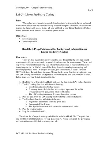
Copyright 2004 – Oregon State University3 of 3The Synthesis functionThe synthesis part is fairly easy compared to the coding function. Fist for eachframe you need to create an initial signal to run through the filter. This initial signal isalso of length 30mSec. Using the information from the variable passed into the synthesisfunction you will be able to synthesize each frame. After you have synthesized theframes you can put them together to form the synthesized speech signal.The initial 30mSec signal in created based on the pitch information. Rememberthat if the pitch is zero, the frame is unvoiced. This means the 30mSec signal needs to becomposed with white noise. (look at the MATLAB function randn) If the pitch is notzero, you need to create a 30mSec signal with pulses at the pitch frequency. (look at theMATLAB function pulstran)Now that you have the initial signals all you have left to do is to filter them usingthe gain and filter coefficients and then connect them together. (look at the MATLABfunction filter)Putting the frames back together is also done in a special way. This is where thereason for having the frames overlap becomes clear. Because each frame has its ownpitch, gain and filter, if we simply put them text to each other after synthesizing them all,it would sound very choppy. By making them overlap, you can smooth the transitionfrom one frame to the next. The figure below shows how the frames are connected. Theamplitude of the tip and tail of each frame’s data is scaled and then simply added.Figure 2: Addition of separate frames into final audio signalInterpreting your resultsThere are several ways to look at the results but for the sake of simplicity we willrely on the human ear. In the main function the input speech audio and the synthesizedspeech audio is played back to back. You can listen to these playbacks and judgeaccordingly if your coding and synthesis functions are working.Post LabWrite a paragraph summarizing what you have learned in this Lab. Also includea copy of all MATLAB code written and a copy of all the plots and images created. Turnin your lab results to your Lab TA at the beginning Lab in three weeks.ECE 352, Lab 5 – Linear Predictive Coding
Copyright 2004 – Oregon State University1 of 1Lab 4 – Filter designIdeaYou work for a forensics investigative company as part of their technical team. Asurveillance tape, linked to the current case, has been found but the camera lens wassmashed so only the sound is good. Because the camera was on the outside of a buildingand the wind was blowing fairly strong it sounds like there is only noise on the tape.Your task now, is to use MATLAB to process the recording to see if you can clean upsome of the noise and find any vital information on the tape.Objectives Analysis of signal spectrumSignal separation through filteringBode plotsProcedureFirst you will need to look at the signal and determine at what frequencies thesignal and noise are. Then you can design a filter that will get rid of the noise signal.Remember, the human ear can only hear up to about 20KHz. Also, the human voicewhen speaking is typically no higher than 5KHz. So, if the noise is above 5KHz you canfilter it out without loosing the data you recorded.Getting the sound data into MATLABTo get the recording into your computer you played it back through the mic injack on your sound card and recorded it with Windows sound recorder. The data is nowstored as a *.wav file.1)In MATLAB, find functions that will read, play, record *.wav files.Make sure that you are able to read in and play back the recorded data beforecontinuing. Look at things like sample rate, and how the sample rate affects what youhear when playing back the data. Try plotting the data to see what it looks like. Is thiswhat you would expect? Explain!Look at frequency spectrumTo find out if the noise can be filtered out you will need to look at the frequencydistribution of the data.2)Do an FFT on the data and plot the results as amplitude vs. frequency.What frequencies are present? What frequencies can you safely say are connectedto the noise? Is there anything in the frequency range for the human voice? Is this whatyou are expecting? Explain!ECE 352, Lab 4 – Filter design
Copyright 2004 – Oregon State University2 of 2Designing a filterWhen designing filters, bode diagrams could be useful. Every transfer functionhas a corresponding bode diagram. Remember the low pass filter from lab2? Its circuitis shown in the figure below.Figure 1The cutoff frequency is set by the values of R and C. If this one filter is notsufficient, multiple of the same filters can be cascaded for better results. Bode diagramsshow the magnitude and phase response of a transfer function. In other words it showsthe gain for different input signal frequencies. When the gain is greater than one for aparticular frequency, the signal will be amplified. When the gain is less than one for adifferent frequency, the signal will be filtered out to the extent of the gain.3)Design a transfer function that will filter out the frequencies that correspond to thenoise in your data.4)Enter the transfer function into MATLAB and verify that the bode diagram iswhat you intended it to be.Look in your textbook at bode plots to try and understand them better. The bode()function in MATLAB requires your transfer function to be in a state space model format.The following lines can be used to create this model. [A,B,C,D] tf2ss(Num,Den); sys ss(A,B,C,D);Where Num is a matrix containing the coefficients of the numerator of your transferfunction and Den is a matrix containing the coefficients of the denominator of yourtransfer function.Applying the filter to your dataNow that you have your filter designed it is time to run your recorded datathrough it. MATLAB has a lot of functions that would allow you to do this. One of themis lsim. This function takes as input a state space model, input signal and input timevector. The output is of the same dimensions as the input signal. Read the help on lsimfor more information5)Use lsim to find the output by running your recorded data through your newlydesigned transfer function.Interpreting your resultsThere are several ways to look at the results. You can look at the FFT of youroutput signal and see if the high frequencies are gone. You could plot your output signalECE 352, Lab 4 – Filter design
Copyright 2004 – Oregon State University3 of 3and compare it to the input signal. You could also play the output signal and hear if thenoise is gone. If the noise is still there you might want to redesign you filter transferfunction.Post LabWrite a paragraph summarizing what you have learned in this Lab. Also includea copy of all MATLAB code written and a copy of all the plots and images created. Turnin your lab results to your Lab TA at the beginning Lab in two weeks.ECE 352, Lab 4 – Filter design
Copyright 2004 – Oregon State University1 of 1Lab 3 – Image processingIdeaIn this lab you are going to use the camera together with MATLAB’s imagingtoolbox to create a change counter. You will take a picture with the camera and then useMATLAB to process the image to find and count the change.Objectives Image processing techniquesMore MATLABProcedureThe concept is fairly easy; when taking a picture of some coins, the picture can beconverted to a black and white image. The black represents the background and thewhite is the coins. The coins in the image can then be labeled and the area of each coincan be calculated. With normalizing the areas of all the coins and then using simpleratios between the different areas, we can distinguish between quarters, dimes, nickelsand pennies. In this lab you will go through these steps to build your change counter.Taking the picture of the coins1)Take a couple of pictures of some change arranged on a table.To prevent unnecessary difficulties with all the different exceptions with buildinga change counter we are going to specify a couple of guidelines for taking the pictures: Each picture may only contain quarters, dimes, nickels and pennies. Each picture must contain at least one quarter. The coins may not overlap or touch each other. Lay the coins on a surface that would provide a good contrast with the coins. Make sure you have good lighting when taking the picture.Finding the coins with MATLABThe hardest part of this project is to accurately change a color picture of the coins,Figure 1, into a black and white picture where the coins are white and the rest is black,Figure 2. (Recall that in an image, black is represented with zeros and white with ones.The assumption is made that background data defaults to zeros while ones representobjects in the foreground)Figure 1ECE 352, Lab 3 – Image processingFigure 2
Copyright 2004 – Oregon State University2 of 2Note, when first taking the picture and converting it to black and white, you willsee that the coins are actually black and the rest is white. This is simply due to the factthat the coins are darker than the white background.Some of the problems that you will encounter are: When taking a picture, due to reflection, some sections on coins will appear justas light as the background. When converting to a black and white image, thecoins will not be solid objects. Figure 3. This could cause inaccurate areacalculations of the coins. Due to inadequate lighting while taking a picture, the corners of your image mightappear darker than the coins. In the black and white image, these corners willalso show up as foreground objects and might be interpreted as coins. Figure 4.Figure 3Figures 41)Figure 2 shows a picture that has been properly converted to a black and whiteimage. This was done by using a combination of MATLAB functions like: RGB2Gray,im2bw, imfilter, and imfill. Write some MATLAB code that would convert a colorimage of coins to a black and white image as described above.Labeling coins and finding areasIn order to distinguish between the different foreground objects in the picture,each object (coin) needs to be labeled. bwlabel does this. After the coins are labeled youneed to figure out how to single out a coin in order to calculate its area. bwarea is afunction that returns the area of all the objects in the foreground.2)Using bwlabel, bwarea or any other MATLAB functions, write some code thatwill process a black and white image and return to a variable an array of areas. The arraywill be the same size as the number of coins in the picture. Each element in the array willcontain the area of its corresponding coin.Ratios between coinsWhen taking a picture of coins, the size of the coins in the picture depends on thedistance the camera is from the coins when taking the picture. Thus the only thing thatremains constant in all the different pictures is the coin size ratios.3)Use this fact and the array of areas to determine what coins are present in theimage. Write some code that will then calculate the value of the change in the picture.ECE 352, Lab 3 – Image processing
Copyright 2004 – Oregon State UniversityPost Lab3 of 3Write a paragraph summarizing what you have learned in this Lab concerningimage processing. Also include a copy of all MATLAB code written and a copy of allthe plots and images created. Turn in you lab results to your Lab TA at the beginning ofthe next Lab session.ECE 352, Lab 3 – Image processing
Copyright 2004 – Oregon State University1 of 1Lab 2 – Sampling, Filters and FFTsIdeaFor this lab you are going look at the effect that a low pass filter has on a signalthat contains a high and low frequency component. Also you are going to use FourierTransforms to look at the effect that different sampling rates and sampling window sizeshave on the frequency composition of signals.Objectives Deriving an impulse response from a circuitEffects of Sampling RateEffects of Sampling window sizeFourier TransformsProcedureFor this lab you are going to construct a signal, x(t), from two cosine waves ofdifferent frequencies. Then you will derive the impulse response from the low pass filtershown in Figure 1. Find the output signal, y(t), of this filter for an input x(t) byconvolving x(t) with the impulse response of the filter. Now you will use a FourierTransform to look at the frequency composition of x(t) and y(t) for different sample ratesand sample window sizes.Figure 1Construct input signal x(t)1)In MATLAB construct a signal that consists of two cosine waves. The first waveshould have a frequency of 100 Hz and the second a frequency of 10 KHz.Sample this signal at double Nyquist rate and with a window size of 5 of the lowfrequency periods. Figure 2.Circuit Output through Convolution2)Derive the impulse response h(t) for the low pass filter circuit shown in Figure 1.In MATLAB, sample h(t) with the same frequency and window size as the signalyou constructed, x(t). Using convolution and the impulse response, find theoutput, y(t), to the filter given x(t) is the input signal. Notice that the highfrequency component should almost all be gone. Figure 2.ECE 352, Lab 2 – Sampling, Filters and FFTs
Copyright 2004 – Oregon State University2 of 2Figure 2Fourier TransformsA Fourier Transform gives you information of the frequency composition of asignal. You are now going to look at the effect of the low pas filter, using FFTs.3)In MATLAB find the function that does a Fourier Transform. Do the FourierTransform on both the input signal, x(t), and the output signal, y(t). Plot thesetransforms as shown below.Figure 3ECE 352, Lab 2 – Sampling, Filters and FFTs
Copyright 2004 – Oregon State University3 of 3You can use your mouse to zoom in on the plot. Look at which frequencies arepresent. Is this what you are expecting? Also pay attention to the x axis of this plot.You will have to construct a vector for the x axis. You are no longer in the time domainso instead of plotting the magnitude against time, you are plotting the magnitude againstfrequency.Sample Rate and Window SizeNow that you have everything set up to produce the two plots shown in Figure1and Figure 2, start playing around with the sample rate and the sample window size.4)5)The sample rate: Rerun your code for a couple of different sample rates. Start atdouble Nyquist rate and then decrease the sample rate. At what point do you startgetting strange frequencies in you plots?Sample window size: Change the sample window size so that you are no longersampling exactly at an inter number of the low frequency period. How does thiseffect the FFT plots for x(t) and y(t)? (Zoom in on the plot to see the effect)Post LabWrite a paragraph summarizing what you have learned in this Lab concerningfilters, sample rates and sample window sizes. Also include a copy of all MATLABcode written and a copy of all the plots and images created. Turn in you lab results toyour Lab TA at the beginning of the next Lab session.ECE 352, Lab 2 – Sampling, Filters and FFTs
Copyright 2004 – Oregon State University1 of 1Lab 1 – MATLAB, usb cam, ConvolutionIdeaDuring this lab you will become familiar with MATLAB and how to use its helpfunction. You will also get to test out the TekBotsTM usb cam using MATLAB. Lastlyyou will also revisit the concept of convolution and write a user defined function inMATLAB involving convolution.Objectives Review MATLAB concepts.Test the TekBotsTM usb cam device.Write custom convolution function for MATLAB.ProcedureMATLAB conceptsIn order to use MATLAB efficiently there are two important functions that youneed to know about. The first one is “help”. By typing “help” at the command prompt inMATLAB, you will see a list of functions that is categorized by topic. Typing “help topic ” will list functions within the specified topic. Typing, “help function ” willdisplay information on the functions themselves. Try typing, “help help”. The secondimportant function is “lookfor”. This function will go through all the description text ofall the different functions in MATLAB and list the functions that contain a word that youspecify. For example, “lookfor multiply” will display a list of all the function that hassomething to do with the multiplication of two variables. Spend some time looking at the help info for the following functions:pi, plot, stem, cos, axisLook for functions that would allow you to do: e(x), x2 or 21) Create a 2.5Sec plot of a sine wave with amplitude of 5 and frequency of 2Hz,Figure1.A. Remember that this is a discrete representation of a sine wave. Look atthe difference between plotting the sine wave with 200, 25, 10 and 5 data points inone period.Figure1.AECE 352, Lab 1 – MATLAB, usb cam, ConvolutionFigure1.B
Copyright 2004 – Oregon State University2 of 2Use the stem function to graph one period of the same sine wave with 25 data pointsper period, Figure1.B. How can the plot function be used to see the discrete datapoints as the stem function shows them?3) Modify your equations from 1) in order to have the sine wave’s amplitude decay from5V at 0Sec to roughly 1V at 2.5Sec. Also show the discrete plot, Figure1.C.2)Figure1.CTekBotsTM usb camThere are several different MATLAB functions that have been developed for theTekBots usb cam. “getpic” is the function that will be used during this lab. Refer toSections 4.1 and 4.2 of the usb cam User Guide for instructions on how to use theusb cam with MATLAB. Review the cam datasheet: usb cam.pdf.Look for functions that would allow you to display and save a RGB image. Also,use “help” or “lookfor” to find information on how to write your own MATLABfunctions.Figure24) Use the TekBots usb cam to read a picture into MATLAB. An image consists of a2x2 matrix of pixels. Each pixel has three bytes of information (Red, Green, Blue).From the picture that you took, build another bigger image that consists of 4 subimages. The first image should be a gray scale of the original, while the other threeECE 352, Lab 1 – MATLAB, usb cam, Convolution
Copyright 2004 – Oregon State University3 of 3are the Red, Green and Blue separated out into individual images, Figure2. Write afunction called separateRGB() that will build this new image and return it as avariable. Below is how your function could be used.Example: In MATLABRGB getpic;// usb cam functionBigIM separate(RGB);// your custom functionImage(BigIM);// MATLAB functionConvolutionRecall that the convolution sum expresses the output of a discrete-time system interms of the input and the impulse response of the system. Look for functions that would allow you to do convolutions.5) Write a MATLAB function called show convolution(signal1, signal2). The functionshould take as input; two discrete time waveforms of any size, compute theconvolution and plot both the input waveforms and the resulting convolution. Thethree plots should be displayed on the same window, one above the other, and havethe same axis scale as shown in Figure3 below.Figure3Post LabWrite a paragraph summarizing what you have learned in this Lab. Also includea copy of all MATLAB code written and a copy of all the plots and images created. Turnin you lab results to your Lab TA at the beginning of the next Lab session.ECE 352, Lab 1 – MATLAB, usb cam, Convolution
MATLAB files. Two of these, the main file and the levinson function, are given to you. The LPC coding function and the Synthesis function are the files that you have to write. Below is an overview list of steps for this lab. 1. Read the *.wav file into MATLAB and pass the data to the LPC c