Transcription
SESUG 2020 – Paper 150Look Up Not Down: Advanced Table Lookups in Base SASJay Iyengar, Data Systems Consultants, Oak Brook, ILJosh Horstman, Nested Loop Consulting, Indianapolis, INABSTRACTOne of the most common data manipulation tasks SAS programmers perform is combining tables through table lookups. Inthe SAS programmer’s toolkit many constructs are available for performing table lookups. Traditional methods for performingtable lookups include conditional logic, match-merging and SQL joins. In this paper we concentrate on advanced table lookupmethods such as formats, multiple SET statements, and HASH objects. We conceptually examine what advantages theyprovide the SAS programmer over basic methods. We also discuss and assess performance and efficiency considerationsthrough practical examples.INTRODUCTIONWithin Base SAS, the two most commonly used table lookup techniques are the DATA step merge, and the Proc Sql join.Most SAS users are quite familiar with these techniques and employ them extensively. In our experience, the DATA stepmerge is considered to be the more complex method, where the Proc Sql join is considered to be more intuitive and userfriendly. For this paper, we define these techniques as traditional table lookup methods. Opinions vary on the performanceand efficiency of these two techniques, for given programming situations. Because of the attention they receive in the SASliterature, and their exclusion from many SAS programming courses, many SAS users aren’t aware of advanced techniquesfor combining input tables or SAS data sets. However, SAS contains advanced capabilities for performing table lookups.More experienced SAS users, especially Certified SAS Programmers are more familiar with table lookup methods.WHAT ARE TABLE LOOKUPS?With the advent of databases, a process was devised for organizing data structures in database objects. Part of this processinvolved deciding how to collect and store large amounts of data within a database. Distinct pieces of information would bestored in separate columns, called fields in database terminology. As databases grew in scale, it became practical andefficient to store data in separate database objects. Databases containing large numbers of variables could store sets ofvariables in unique tables. This was the idea of the relational database. Specific variables could be retrieved from theirrespective tables by linking to their table. This is the basic concept of a table lookup.In terms of the structure of a table lookup, a table lookup is performed when two or more data sets are combined horizontally.Table is just an informal name for a SAS data set. The tables are joined based on the value of a key variable or primary key.Each table is indexed on a primary key, which is common to both data sets. Technically, the primary key should be a way touniquely identify records in a data set. For example, many healthcare data sets, use Patient ID as a primary key. In a DATAstep Merge, the primary key is the BY variable, specified in a BY statement. In a Proc Sql join, the primary key is the variablespecified in a join condition in the WHERE or ON clause.Amongst SAS users, table lookups have been used interchangeably with merges and joins. In the simple example of a tablelookup, you have a Base table which contains the bulk of your data, and a lookup table which contains only a few variables.The Base table can be thought of as a master data set containing millions of records or observations, where the lookup tableis usually much smaller. This example of a table lookup is directly relevant to healthcare data sets which can be verymassive. Healthcare data sets may contain millions of patient records, and codes to indicate medical diagnoses orprocedures. They must be linked to smaller reference tables to obtain the code definitions. Figure 1 displays a schematicof a table lookup with five tables.1
Figure 1. Table Lookup SchemaMETHODS FOR TABLE LOOKUPSThere are many methods available for performing table lookups using Base SAS software, ranging from the simple to thecomplex. Carpenter (2001 and 2015) details several such methods.Selecting a method to use for a given situation may depend on a number of factors. When dealing with large data sets,efficient performance may be a priority. In other cases, it may be desirable to keep the code as simple as possible for easeof maintenance and reuse. Each table lookup method has its own advantages and disadvantages, which must beconsidered in the context of the task being performed.It is advantageous for the SAS programmer to be familiar with a variety of methods. Although this paper focuses on severalmore advanced techniques, we begin with a review of several simple approaches commonly used.SIMPLE TABLE LOOKUP METHODSAt its core, a table lookup is simply retrieving a value for one variable based on the value for another. One of the simplestmethods for accomplishing this is by hard-coding the relationship between the two variables directly into the programminglogic. This is often done through a series of IF THEN ELSE statements or a SELECT statement. Horstman (2017)presents a method for hard-coding a table lookup using the WHICHC/WHICHN and CHOOSEC/CHOOSEN DATA stepfunctions. These approaches are quick and easy when the lookup values are few in number and unlikely to change, but theydo not scale well.Another way of performing a table lookup is by combining multiple data sets using the MERGE statement in the DATA step.This is a very common approach because it is simple and versatile. However, it does have some limitations. One notabledrawback is that data sets must generally be sorted before they can be merged in this manner. When data sets are large,sorting can be a costly operation. In addition, there are other pitfalls associated with the DATA step merge. Horstman(2018) details several potential problems.SQL joins are another common means of accomplishing a table lookup. One advantage of a SQL join over a DATA stepmerge is that there is typically no need to sort the incoming data sets prior to a SQL join. Thus, the table lookup can becompleted with a minimal amount of code. However, SQL joins can be quite resource-intensive in certain situations.ADVANCED TABLE LOOKUP METHODSAlthough the simple table lookup methods listed above are sufficient for the majority of programming tasks, there aresituations when a more advanced procedure can be advantageous. This paper examines the following five methods:2
1. Formats2. Hash Tables3. Multiple SET Statements4. Indexes with the KEY Option5. Arrays and the DOW LoopMETHOD #1: FORMATSOne of the traditional and basic ways to perform a table lookup is to use SAS Formats. Although his is a basic technique,we’ve chosen to explore FORMATS because they present an alternative to the commonly used DATA step merge, andPROC SQL join. Thus for the purposes of this paper, FORMATS will be treated as an advanced lookup technique.To perform a table lookup using formats, the SAS user creates a user-defined format using PROC FORMAT. Theprogrammer has two options. The key values and the data values of a user-defined format can be coded explicitly in a PROCFORMAT VALUE statement, or based on variables in a SAS data set. Thus, the lookup table may not be a table at alldepending on the method chosen. If the programmer creates the format from a SAS data set, the data set must have aspecific structure containing key values and data values. Conversely, the lookup values need to be specified directly in thecode, and hard-coded and mapped to key values in the PROC FORMAT step.PROC FORMAT WITH PUT FUNCTION/* Map Race Code to Racial Description */Proc Format;Value RaceEth1 'White'2 'Black'3 'Hispanic'5 'Asian Pacific Islander';NOTE: Format RACEETH has been output.Run;NOTE: PROCEDURE FORMAT used (Total process time):real time0.06 secondscpu time0.03 seconds/* Derive New Variable containing Race Description */Data CARRIER CLAIM 2010;Set SASDATA1.CARRIER CLAIM 2010;RaceEth Description Put(Race, RaceEth.);Run;NOTE: There were 1163957 observations read from the data set SASDATA1.CARRIER CLAIM 2010.NOTE: The data set WORK.CARRIER CLAIM 2010 has 1163957 observations and 14 variables.NOTE: DATA statement used (Total process time):real time3.86 secondscpu time1.54 secondsFigure 2. Proc Format and DATA step using Put Function.3
In the example in Figure 2, a user-defined format RACEETH is created in the first step using PROC FORMAT. RACEETHassigns descriptive labels for racial categories to numeric values. The format is defined as numeric because the key valuesare numeric, which are assigned to character data values. The format specifies a limited, small number of values and labels.This is typical for demographic variables which are commonly discrete or nominal, as opposed to continuous.In the second step, a DATA step reads the SAS data set CARRIER CLAIM 2010, which contains Medicare claims data for2010. CARRIER CLAIM 2010 is our Base table. As indicated in the SAS log, it’s a large data set, containing 1,163,957records. RACE is a variable in CARRIER CLAIM 2010 which contains numeric codes. As we stated earlier, administrativehealthcare data sets contain codes to indicate diagnoses, procedures, physicians, etc.In this case, the format RACEETH contains the lookup values, instead of the values being stored in a separate table.The lookup is performed by applying the newly created format to the RACE variable, and storing the result in a new variable.An assignment statement and a PUT function are used to create the RACEETH DESCRIPTION variable. The formatRACEETH is included as an argument in the PUT function and applied to RACE.One drawback of this technique is that it requires a lot of maintenance for larger sets of data values. A demographic variablesuch as race is well-suited to this technique, because it contains a small number of distinct values. If the set of values were inthe hundreds, imagine how tedious and arduous a task it would be for the programmer to hard-code all those unique values.Also suppose that the values need to be updated or values need to be added to the format. In this case, the programmerneeds to manually modify and edit the hard-coded values. This takes the risk that typos or mistakes will be made whichmight compromise the validity of the data.In this example, the format with a PUT function method executed efficiently. In terms of performance, the table lookupprocessed in a very short amount of time with a base table containing over a million records. The log in Figure 1 shows theexecution took less than 4 seconds of real time, and under 2 seconds of CPU. However, the technique has the disadvantageof maintainability, because it requires manual editing. Similarly, it isn’t practical with a large volume of lookup values. A bettersolution would be to utilize a data-driven technique.PROC FORMAT CNTLIN SAS DATA SETIn our previous example, we concluded the PROC FORMAT and PUT function method was inappropriate for tablelookups where the unique lookup values were in the hundreds or thousands. For example, administrative healthcaredata sets contain ICD9 or ICD10 diagnosis codes. There can be as many as 15,000 to 17,000 individual ICD9 orICD10 diagnosis codes. Using the CNTLIN option in PROC FORMAT, SAS has versatile capabilities for creatingformats to cope with such a large volume of data values. With this construct, SAS can perform effective table lookupswhere the lookup values are on a large scale.SAS can create a format from a SAS data set which contains the lookup values. In PROC FORMAT, you need tospecify the SAS data set using the CNTLIN option. There are several requirements for a CNTLIN data set. It needsto contain several variables. START contains the values in a VALUE statement from the left side of the equals sign.LABEL contains the values from the right-side of the equal sign or the lookup values.In Figure 2 below, the excerpt from the SAS log illustrates a DATA step which manipulates the SAS data set, ICD9DX. Thedata set ICD9DX contains over 17,300 unique medical diagnosis codes. The required variables for a CNTLIN data set areSTART, LABEL, and FMTNAME. The DATA step prepares ICD9DX to meet the requirements of a CNTLIN data set. TYPE,which is assigned ‘C’, is an optional variable which indicates the type of format, character or numeric. For a format based ona range of numeric values, an additional variable, END, would be needed.4
/* Preparing the CNTLIN SAS Data Set */Data ICD9DX;Set advtbllu.icd9dx(Rename (Description Label));Retain Fmtname ' ICDDX' Type 'C';Start Compress(code, '.');Keep Type Start Label Fmtname;Run;NOTE: There were 17374 observations read from the data set ADVTBLLU.ICD9DX.NOTE: The data set WORK.ICD9DX has 17374 observations and 4 variables.NOTE: DATA statement used (Total process time):real time0.03 secondscpu time0.02 secondsProc Format Cntlin ICD9DX;NOTE: Format ICDDX has been output.Run;NOTE: PROCEDURE FORMAT used (Total process time):real time0.19 secondscpu time0.18 secondsNOTE: There were 17374 observations read from the data set WORK.ICD9DX.Data carrier claim 2010;Set advtbllu.carrier claim 2010;DX1 Put(ICD9 DGNS CD 1, ICDDX.);Run;NOTE: There were 1163957 observations read from the data set ADVTBLLU.CARRIER CLAIM 2010.NOTE: The data set WORK.CARRIER CLAIM 2010 has 1163957 observations and 10 variables.NOTE: DATA statement used (Total process time):real time2.97 secondscpu time2.64 secondsFigure 3. DATA step to prepare CNTLIN data set and Proc Format with CNTLIN option.In the SAS log in Figure 3 above, SAS creates and outputs the format, ICDDX based on the data set ICD9DX. The data setICD9DX contains both the key and lookup values which are stored in ICDDX once it’s created. The coding for the PROCFORMAT CNTLIN is very simple. Once again, the table lookup is executed by applying the format to a variable,ICD9 DGNS CD 1, on the CARRIER CLAIM 2010 using the PUT function, and storing the result in the newly createdvariable, DX1, using a simple assignment statement.In performance, PROC FORMAT CNTLIN matched if not exceeded the efficiency of the previous technique. As shown inFigure 3, the execution took less than 3 seconds of real time, and under 3 seconds of CPU. Our example demonstrates thesuitability of this method to handle large lookup tables. Also, the technique has the advantage of providing a data drivensolution to a table lookup. If changes need to happen to the data, they can happen at the data set level, without lots ofmanual intervention by the programmer at the code level.5
METHOD #2: HASH TABLESWHAT ARE HASH TABLESThe hash object has been available in the Base SAS package since version 9. Hash tables are lookup tables defined usinghash objects. Hash objects are commonly referred to as hash tables. Technically, the hash object is a DATA step componentobject consisting of attributes and methods. The hash object must be declared and instantiated within a DATA step. Oncedefined, hash objects are stored in memory for the duration of the DATA step, while data values are accessed and retrievedfrom the table. Thus, hash tables use in-memory processing, as opposed to disk-based processing.The tabular structure of a hash object is similar to a SAS data set, and contains rows and columns. The hash table containsa key component and a data component, analogous to key values and data values respectively. The key values must beunique and serve as an index or primary key for mapping to the data values. Key and data variables can be single, orcomposite, consisting of multiple variables, and allow storage of multiple key and data values. The hash table has theversatile feature of allowing key and data variables to be character, numeric or a mixture of the two. Data loaded into a hashobject can be hard-coded in a DATA step, or loaded directly from a SAS data set. Unlike a DATA step merge, a hash tablelookup doesn’t require data to be sorted or indexed prior to processing.HASH TABLE CODINGIn the DECLARE HASH statement, the hash object is invoked, the hash table is given a name, and dimensions for the hashtable are defined. If the hash table is loaded from a SAS data set, it’s specified in parentheses and double quotes as shownbelow. If this is the case, it’s not necessary to explicitly define the hash table dimensions in terms of rows and columns.Otherwise, the number of buckets or total cells for the hash table needs to be specified in parentheses.Declare Hash ‘Hash Table Name’ (“libref.sasdatasetname”);.The next sets of statements initialize the variables that the declared hash table will contain. The DefineKey method definesthe key variables of the hash table, which serves as a primary key, and indexes the hash table. The key variables arespecified in parentheses and double-quotes. The key variables can be taken from the SAS data set which the hash table isbased on.HashTableName.DefineKey (“Key Variable(s)”);The DefineData property method defines the data component of the hash table. The data variable contains the actual lookupvalues we’re interested in. The data variable is specified in parentheses and double-quotes, and can be taken from the SASdata set which populates the hash table. There can be multiple data variables defined within the hash table.HashTableName.DefineData (“Data Variable(s)”);The DefineDone property method completes the declaration of the hash table. It indicates that the dimensions, SAS dataset, and variables have all been specified. The End statement concludes the block of code which defines the hash table.HashTableName.DefineDone;End;6
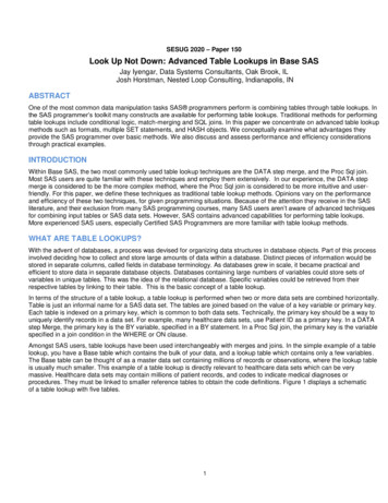
DATA STEP PROCESSING USING HASH TABLESIt is important to understand how a HASH object processes and performs a table lookup. To understand this, it’s necessaryto look behind the scenes at what SAS is doing when it executes code. One of the internal constructs which the DATA stepuses is the Program Data Vector (PDV). The PDV holds one record of data at a time as it’s processed by DATA step codeduring each iteration or loop of the DATA step. The following diagram shows what happens to the PDV as each line of DATAstep code is executed in a hash table lookup operation.Data BENE MATCH BENE NO MATCH;If 0 Then Set sasfiles.finder attrib;PDVBENE IDPRFNPIEOF1CLM ID0RCERRORN.01Figure 4. Set Statement and PDVThe first line of code is a non-executing SET statement. When you specify ‘IF 0 Then Set’, SAS compiles the SET statement,and adds the variables contained in the data set FINDER ATTRIB to the PDV. If it was an executing SET statement, thePDV would be populated with the first record of data from FINDER ATTRIB. Instead SAS initializes variables to missing. Thevariables from the other SAS data set have been added to the PDV as well. In addition the PDV contains any temporaryvariables defined during the step (EOF1), and the automatic variables, ERROR and N . The variable N counts DATAstep iterations.If N 1 Then Do;Declare Hash Provider (dataset: 'sasfiles.finder attrib');Provider.DefineKey ('BENE done ();End;PDVBENE IDPRFNPIEOF10CLM IDRCERRORN.01Figure 5. Hash Object Creation and PDV.In the next step, SAS initializes and declares the hash object only in the first iteration of the DATA step (IF N 1).The hash object is created in memory. The hash table, PROVIDER, is loaded with data from the data set,SASFILES.FINDER ATTRIB. Key and data variables are defined for the PROVIDER hash table. No changes occur in thePDV, because the hash table resides in memory and doesn’t require any data processing to take place. Nothing from thehash object is added to the PDV.7
Do Until (EOF1);Set sasfiles.carrier2010 end EOF1;PDVBENE IDPRFNPIEOF1CLM e 6. Second SET statement executesInside the DO Loop, SAS executes the SET statement and reads the data set SASFILES.CARRIER2010. The temporaryvariable EOF1 is defined using the END option. The first observation in SASFILES.CARRIER2010 is read and loaded intothe PDV. The data set SASFILES.CARRIER2010 actually contains many more variables than can be shown here. The fulldata set is listed in the appendix.Call Missing (PRFNPI);PDVBENE IDPRFNPIEOF1CLM e 7. CALL MISSINGThe CALL MISSING routine initializes the values of the Lookup variable PRFNPI to missing.Do Until (EOF1);Set sasfiles.carrier2010 end EOF1;Call Missing (PRFNPI);RC Provider.find();PDVBENE IDPRFNPIEOF1CLM 41001Figure 8. The Find Method8
Using the FIND Method, SAS searches the hash table PROVIDER using BENE ID as the key variable, and the value ofBENE ID from the first record of SAS data set CARRIER2010 that’s in the PDV. A match in the hash table PROVIDER isfound, and SAS populates PRFNPI in the PDV from the value in the hash table. The variable RC (Return Code) is createdand indicates the result of the FIND Method. Its assigned RC 0 because the FIND Method successfully found a match.Do Until (EOF1);Set sasfiles.carrier2010 end EOF1;Call Missing (PRFNPI);RC Drgcode.find();If RC 0 Then Output BENE MATCH;PDVBENE IDPRFNPIEOF1CLM 41001Figure 9. Output to SAS data set.Because the FIND Method was successful (RC 0), an IF-THEN statement writes the record in the PDV to the output dataset, BENE MATCH. This ends the first iteration of the DATA step.HASH TABLE EXAMPLESThe Data SetThe data sets used for this hash table example comes from the GDELT (Global Database of Events, Language, and Tone)Project. The GDELT Project built a worldwide database of international conflicts and interactions between countries aroundthe world. The database stores records of events covered by different media networks and news outlets. It was compiledfrom hundreds of print, broadcast, and online news sources. The full database consists of 250 million historical recordsdating back from the present day to 1979, and is updated periodically. For the examples using hash tables, a subset of thefull database was used. This subset was used as the base table in our hash table example. A PROC CONTENTS of theGDELT data set is provided in the appendix. A snapshot of the GDELT data set is displayed in Figure 10 LI NG LI NG ANG ZEMINCHNCHINA439.2307692311140913619930101CHNGOVLI NACHNCHINA10013.22645291Figure 10. GDELT data setThe lookup table for this hash table example is much smaller and contains Event Descriptions for the Event Codes in thebase table. A sample of the lookup table is provided in Figure 11 below.9
CAMEOEVENTCODE1101112131415hEVENTDESCRIPTIONMAKE PUBLIC STATEMENTMake statement, not specified belowDecline commentMake pessimistic commentMake optimistic commentConsider policy optionAcknowledge or claim responsibilityFigure 11. Event Code Lookup TableA series of tests were run on the data sets using the hash table lookup method. The tests were performed using SASUniversity Edition version 3.8. SAS University Edition is run on a virtual machine which contains system resources. Thevirtual machine has 3.5 GB of random-access memory (RAM), and 11.5 GB of storage space. SAS University Edition isknown to freeze or crash when the number of observations exceeds 10 million. This is due to storage space or spaceallocation limitations for output data sets. As a result, the amount of data read from the base table was limited to 5 millionobservations.Data CODE MATCH CODE No Match;If 0 Then Set cameo event codes;IF N 1 Then Do;Declare Hash CODE (dataset: 'cameo event codes');CODE.DefineKey ('EVENTCODE');CODE.DefineData ('EVENTDESCRIPTION');CODE.DefineDone();End;Do Until (EOF1);Set advtbllu.gdelt all(obs 5000000) End EOF1;Call Missing (EVENTDESCRIPTION);RC CODE.Find();IF RC 0 Then Output CODE MATCH;Else IF RC 0 Then Output CODE No Match;End;Run;NOTE:NOTE:NOTE:NOTE:NOTE:There were 299 observations read from the data set WORK.CAMEO EVENT CODES.There were 5000000 observations read from the data set ADVTBLLU.GDELT ALL.The data set WORK.CODE MATCH has 4998980 observations and 11 variables.The data set WORK.CODE NO MATCH has 1020 observations and 11 variables.DATA statement used (Total process time):real time14.92 secondscpu time7.95 secondsFigure 12. hash table-Table LookupThe hash table lookup example in Figure 12 illustrates a many-to-one merge. The base table contains duplicate records fordistinct values of the key variable EVENTCODE. The lookup table contains a single record for each unique value ofEVENTCODE. The OBS option was used to limit the number of observations read and processed from the base table to5000000. The lookup table with event code contains 300 observations.10
The output of the table lookup includes separate data sets for matches and non-matches based on the return code. Asindicated Figure 12, the SAS log shows the execution of the table lookup completed in less than 15 seconds of real time. Inorder to assess relative efficiency of the hash table technique, this exercise was repeated using conventional table lookuptechniques. The example was repeated using the common DATA step merge and PROC SQL join constructs./* Data Step Merge Example */Proc Sort Data advtbllu.gdelt all(Obs 5000000) Out GDELT ALL;By EVENTCODE;Run;NOTE: There were 5000000 observations read from the data set ADVTBLLU.GDELT ALL.NOTE: PROCEDURE SORT used (Total process time):real time21.88 secondscpu time18.05 secondsProc Sort Data advtbllu.cameo event codes(Rename (cameoeventcode eventcode))out cameo event codes Nodupkey;By EVENTCODE;Run;NOTE: The data set WORK.CAMEO EVENT CODES has 299 observations and 2 variables.NOTE: PROCEDURE SORT used (Total process time):real time0.63 secondscpu time0.03 secondsData AdmHlth.gdelt all v2;Merge gdelt all (IN A) cameo event codes (IN B);By EVENTCODE;If A and B;Run;NOTE:NOTE:NOTE:NOTE:There were 5000000 observations read from the data set WORK.GDELT ALL.There were 299 observations read from the data set WORK.CAMEO EVENT CODES.The data set ADMHLTH.GDELT ALL V2 has 4998980 observations and 10 variables.DATA statement used (Total process time):real time30.24 secondscpu time6.42 secondsFigure 13. DATA step Merge Table LookupIn Figure 13 above is the SAS log from the retest of the same example using the DATA step merge. Repeating the examplewith the DATA step merge resulted in a total execution time of 52.75 seconds of real time, and 24.75 seconds of CPU, asdisplayed in Figure 13. This is three times the amount of CPU time and over three times the amount of real time it took toexecute the table lookup using hash tables. CPU time is appropriate as a metric of efficiency here because both tests wereperformed using the same platform and system.Figure 14 displays the SAS log from a retest using a PROC SQL join. A third run of the same example using a PROC SQLinner join resulted in an execution of 35.58 seconds of real time, and only 8.14 seconds of CPU, as shown in Figure 14. Still,the hash table method performed better in terms of real time, although the results of CPU time were practically the same.11
/* Proc Sql Join Example */Proc Sql INOBS 5000000;Create Table gdelt All V2 asSelect A.*, B.EventDescriptionFrom advtbllu.gdelt all as A, cameo event codes as BWhere A.EventCode B.EventCode;NOTE: Table WORK.GDELT ALL V2 created, with 4998980 rows and 10 columns.Quit;NOTE: PROCEDURE SQL used (Total process time):real time35.58 secondscpu time8.14 secondsFigure 14. DATA step Merge Table LookupTo assess the efficiency as the volume of data increases, additional tests were conducted using the GDELT ALL data set atlarger sample sizes of 8 million and 12 million observations. The tests were conducted using each of the three table lookupmethods; DATA step merge, PROC SQL join, and hash table lookup. As shown in Table1 below, in real time, the hash tablewas the most efficient at sample sizes of 5 million and 12 million observations.DATA step MergeProc Sql JoinHash Table5000000 Obs52.7535.5814.928000000 Obs45.716.0420.4112000000 Obs1:54.7348.2530.39Table 1. Real time Performance Comparison: Intermediate methods vs. Hash TableThe results in CPU time are displayed in Table 2. In CPU time, there was no performance improvement of using the hashtable instead of the PROC SQL join. However, there was a large gap between each of these two techniques, and theresource-intensive DATA step merge. This is due in part to running the time-consuming SORT procedure on the base table.The most striking difference between the hash table and DATA step merge came at the sample size of 12 millionobservations.DATA step MergeProc Sql JoinHash Table5000000 Obs24.758.147.958000000 Obs37.1511.4711.9012000000 Obs56.5518.6818.41Table 2. CPU time Performance Comparison: Intermediate methods vs. hash table12
METHOD #3: MULTIPLE SET STATEMENTSAnother method for performing a table lookup is using a DATA step with multiple SET statements. This is conceptuallysimilar to performing a DATA step merge, but the MERGE statement is not used. This allows the programmer to take directcontrol of the process of matching up records based on the value of one or more key variables. It also has the potential todramatically reduce processing time when compared with the use of the MERGE statement.It is important to note that this method still requires the input data sets be sorted. As in the traditional merge, we will bestepping through each data set sequentially, reading each record only once.A SIMPLE ANALOGYImagine you are given two alphabetized stacks of books. Your
Aug 13, 2019 · the SAS programmer’s toolkit many constructs are available for performing table lookups. Traditional methods for performing table lookups include conditional logic, match-merging and SQL joins. In this paper we concentrate on advanced table lookup methods su