Transcription
ME 304CONTROL SYSTEMSMechanical Engineering Department,Middle East Technical UniversityRadar DishArmaturecontrolleddc motorOutsideθD outputInsideθr inputpθmGearboxControlTransmitterθDdc amplifierME 304 CONTROL SYSTEMSControlTransformerProf.Prof Dr.Dr Y.Y Samim ÜnlüsoyProf. Dr. Y. Samim Ünlüsoy1
CH IXCOURSE OUTLINEI.II.III.INTRODUCTION & BASIC CONCEPTSMODELING DYNAMIC SYSTEMSCONTROL SYSTEM COMPONENTSIV.V.VI.VII.VIII.STABILITYTRANSIENT RESPONSESTEADY STATE RESPONSEDISTURBANCE REJECTIONBASIC CONTROL ACTIONS & CONTROLLERSIX.FREQUENCY RESPONSE ANALYSISX.XI.SENSITIVITY ANALYSISROOT LOCUS ANALYSISME 304 CONTROL SYSTEMSProf. Dr. Y. Samim Ünlüsoy2
FREQUENCY RESPONSE - OBJECTIVESIn this chapter : A short introduction to the steadystate responsepof control systemsytosinusoidal inputs will be given.Frequency domain specifications fora control system will be examined.Bode plots and their constructiong asymptoticy papproximationsppusingwill be presented.ME 304 CONTROL SYSTEMSProf. Dr. Y. Samim Ünlüsoy3
FREQUENCY RESPONSE – INTRODUCTIONNiseNi ChCh. 10 In frequency response analysis of controlsystems, the steady state response of thesystem to sinusoidal input is of interest.The frequency response analyses arecarried out in the frequencyqy domain,domain,rather than the time domain.It is to be noted that, time domainproperties of a control system can bepredicted from its frequency domaincharacteristics.characteristicsME 304 CONTROL SYSTEMSProf. Dr. Y. Samim Ünlüsoy4
FREQUENCY RESPONSE - INTRODUCTION For an LTI system the Laplace transformsoff theth inputit andd outputt t are relatedl t d tot eachhother by the transfer function, T(s).Laplace DomainInput R(s)T(s)C(s)OutputInI theth frequencyfresponse analysis,l i thethsystem is excited by a sinusoidal input offixed amplitude and varying frequency.frequency.ME 304 CONTROL SYSTEMSProf. Dr. Y. Samim Ünlüsoy5
FREQUENCY RESPONSE - INTRODUCTION Let us subjectja stable LTI systemyto asinusoidal input of amplitude R andfrequencyqyω in time domain.r(t) Rsin(ωt) The steady state output of the system willbe again a sinusoidal signal of the samefrequency,, but probably with a differentfrequencyamplitude and phase.phase.c(t) Csin(ωt φ)ME 304 CONTROL SYSTEMSProf. Dr. Y. Samim Ünlüsoy6
FREQUENCYQRESPONSE - INTRODUCTIONME 304 CONTROL SYSTEMSProf. Dr. Y. Samim Ünlüsoy7
FREQUENCY RESPONSE - INTRODUCTION To carryy out the same processpin thefrequency domain for sinusoidal steadystate analysis, one replaces the Laplacevariablei bl s withi hs jjωin the input output relationC(s) T(s)R(s)C(s) T(s)R(s)with the resultC(jω) T(j) T(jω)R(jω)ME 304 CONTROL SYSTEMSProf. Dr. Y. Samim Ünlüsoy8
FREQUENCY RESPONSE - INTRODUCTION The input, output, and the transferfunction have now become complex andthus they can be represented by theirmagnitudes and phases. Input :R(jω) R(jω) R(jω) Output :C(jω) C(jω) C(jω)C(jω)TransferFunction :T(jω) (j ) T(jω)(j ) Τ(jω)(j ) ME 304 CONTROL SYSTEMSProf. Dr. Y. Samim Ünlüsoy9
FREQUENCY RESPONSE - INTRODUCTION With similar expressions for the inputandd ththe ttransferfffunction,tiththe iinputtoutput relation in the frequencydomain consists of the magnitude andphase expressions :C(jω) T(jω)R(jω)C(jω) T(jω)(jω) R(jω)(jω) C(jω) T(jω) R ( jω)ME 304 CONTROL SYSTEMSProf. Dr. Y. Samim Ünlüsoy10
FREQUENCY RESPONSE - INTRODUCTION For the input and output described byr(t) Rsin(ωt)c(t) Csin(ωt φ)the amplitude and the phase of theoutput can now be written asC R T(jω)φ T(jω)T(jω)ME 304 CONTROL SYSTEMSProf. Dr. Y. Samim Ünlüsoy11
FREQUENCY RESPONSE Consider the transfer function for thegeneral closed loop system.systemC(s)G(s)T(s) R(s) 1 G(s)H(s)For the steady state behaviour,behaviour insert s jω.C(jω)G(jω)T(jω)) R(jω) 1 G(jω)H(jω)T(jω) is called the Frequency ResponseFunction (FRF) or Sinusoidal TransferFunction.FunctionME 304 CONTROL SYSTEMSProf. Dr. Y. Samim Ünlüsoy12
FREQUENCY RESPONSE The frequency response function can bewritten in terms of its magnitude andphase.T(jω)) T(jω) T(jω)Since this function is complex,p, it can alsobe written in terms of its real andimaginary parts.T(jω) Re [ T(jω)] jIm[ T(jω)]ME 304 CONTROL SYSTEMSProf. Dr. Y. Samim Ünlüsoy13
FREQUENCY RESPONSE RememberRbthatth t forfa complexlnumberbbebexpressed in its real and imaginary parts :the magnitude is given by :z z a bj( a bj)( a - bj) the phase is given by :22a b-1 b z z tanME 304 CONTROL SYSTEMSProf. Dr. Y. Samim Ünlüsoya14
FREQUENCYQRESPONSE The magnitude and phase of thefrequency response function aregiven by :G(jω)G(jω)T(jω) 1 G(jω)H(jω) 1 G(jω)H(jω) T(jω) G(jω) - [1 G(jω)H(jω)]These are called the gain and phasecharacteristics.ME 304 CONTROL SYSTEMSProf. Dr. Y. Samim Ünlüsoy15
FREQUENCY RESPONSE – Examplep 1a For a system described by thediffdifferentialti l equationti 2x y(t)xdetermine the steady state responsexss(t) for a pure sine wave inputy(t) 3sin(0.5t)ME 304 CONTROL SYSTEMSProf. Dr. Y. Samim Ünlüsoy16
FREQUENCY RESPONSE – Examplep 1b The transfer function is given byX(s)1T(s) Y(s) s ( s 2 ) 2x y(t)xInsert s jω to get :For1T(jω) jω ( jω 2 )ω 0.50 [rad/s]:[ d/ ]11T(0.5j) 0.5j ( 0.5j 2 ) -0.25 jME 304 CONTROL SYSTEMSProf. Dr. Y. Samim Ünlüsoy17
FREQUENCY RESPONSE – Examplep 1c Multiply and divide by the complex conjugate. -0.25 - j 1-0.25 - jT(0.5j) -0.25 j -0.25 - j 1 0.0625T(0.5j) -0.235 - 0.941j Determine the magnitude and the angle.T(0.5j) cos - cos sin sin 76ocos sin -cos sin -2( -0.235 )2 ( -0.941) 0.97-11 T(0.5j)T(0 5j) tant-0.9410.941 -104104o-0.235-104oME 304 CONTROL SYSTEMSProf. Dr. Y. Samim Ünlüsoy18
FREQUENCY RESPONSE – Examplep 1d The steady state response is then given by :(xss (t) 3 ( 00.9797 ) sin 00.5t5t -104104o( 2.91sin 0.5t -104oME 304 CONTROL SYSTEMSProf. Dr. Y. Samim Ünlüsoy))19
FREQUENCYQRESPONSE – Examplep 2a Express the transfer function (input : F,output : y) in terms of its magnitude andphase. cy ky FmyFkcmFME 304 CONTROL SYSTEMSyG(s) 12ms cs kProf. Dr. Y. Samim Ünlüsoy20
FREQUENCYQRESPONSE – Examplep 2b Insert s jω in the transfer function toobtain the frequency response function.G(s) T(jω) 12m ( ωjj) c ( ωjj) k (1ms2 cs k1)k - mω2 cωj jWriteW i theh FRF iin a bjbj form.fME 304 CONTROL SYSTEMSProf. Dr. Y. Samim Ünlüsoy21
FREQUENCYQRESPONSE – Examplep 2c Multiply and divide the FRF expression withthe complex conjugate of its denominator.()()T(jω) 22222kmω cωjkmωcωj()()kmω cω()()k - mω2 - cωj1(k - mω2 - cωj) 2kmω cω-cωT(jω) j22 k - mω2 ( cω )2 k - mω2 ( cω )2 ()()T(jω) Re [ T(jω)] Im[ T(jω)] jME 304 CONTROL SYSTEMSProf. Dr. Y. Samim Ünlüsoy22
FREQUENCYQRESPONSE – Examplep 2d Obtain the magnitude and phase of thefrequency response function.z a2 b2T(jω) ((k - mω))22 ( cω )2 2 2 ( cω ) k - mω b z tan-1aME 304 CONTROL SYSTEMS22 1(2k - mω-1 T(jω) tanProf. Dr. Y. Samim Ünlüsoy)2(2 ( cω )-cωk - mω223)
FREQUENCYQRESPONSE – Examplep 3a The open loop transferfunction of a controlsystem is given as :G ( s) 300 ( s 100 )s ( s 10 )( s 40 )Determine an expression for the phase angleof G(jw)(j ) in terms of the anglesgof its basicfactors. Calculate its value at a frequency offactors28.3 rad/s.Determine the expression for the magnitudeof G(jw) in terms of the magnitudes of itsbasic factors . Find its valueal e in dB at afrequency of 28.3 rad/s.ME 304 CONTROL SYSTEMSProf. Dr. Y. Samim Ünlüsoy24
G ( s) 300 ( s 100 )FREQUENCY RESPONSE– Example 3bs ( s 10 )( s 40 ) G(jω) 300 G(jω 100) - G(jω) - G(jω 10) - G(jω 40)-1 ω -1 ω -1 ω -1 ω 0 tan - tan - tan - tan 100 0 10 40 -1 ω o-1 ω -1 ω 0 tan - 90 - tan - tan 100 10 40 oo-1 28.3 G(28.3j) 0 tan o-1 28.3 -1 28.3 - 90 - tan - tan 100 10 40 0o 15.8o - 90o - 70.5o - 35.3o -180oME 304 CONTROL SYSTEMSProf. Dr. Y. Samim Ünlüsoy25
G ( s) 300 ( s 100 )s ( s 10 )( s 40 )G ( jω ) FREQUENCY RESPONSE– Example 3c300 jωj 100jω jω 10 jω 40222ω 40300 ω 1002ω ω 10222300 2828.33 100G ( 28.3j ) 228.3 28.3 1022228.3 40( 300 )(103.9 ) 0.749( 28.3 )( 30.0 )( 49.0 )ME 304 CONTROL SYSTEMSProf. Dr. Y. Samim Ünlüsoy262
FREQUENCY RESPONSE Typical gain and phase characteristics of aclosed loop system. T(jw) T (jω)0Mr10.707ωrME 304 CONTROL SYSTEMSBWωProf. Dr. Y. Samim Ünlüsoyω27
FREQUENCYQDOMAIN SPECIFICATIONS Similar to transient responsespecifications in time domain,frequency response specifications aredefined.- Resonant peak, Mr,- Resonant frequency, ωr,- Bandwidth, BW,- Cutoffff Rate.ME 304 CONTROL SYSTEMSProf. Dr. Y. Samim Ünlüsoy28
FREQUENCYQDOMAIN SPECIFICATIONS Resonant ppeak, Mr :peak,This is the maximum value of thetransfer function magnitude T(jω) . T(jω) Mr1Mr depends on the damping ratioξ only and indicates the relativestability of a stable closed loopsystem.A large Mr results in a largeovershoot of the step response.As a rule of thumb, Mr should bebetween 1.1 and 1.5.ME 304 CONTROL SYSTEMSProf. Dr. Y. Samim ÜnlüsoyωωrMr 12ξ 1 - ξ229
FREQUENCYQDOMAIN SPECIFICATIONS ResonanttRfrequency,, ωr :frequency T(jω) Mr1This is the frequencyat which the resonantpeak is obtained.ωr ωn 1 -2ξ2ωrωNote that resonant frequency is different than both theundampedpand dampedpnatural frequencies!qME 304 CONTROL SYSTEMSProf. Dr. Y. Samim Ünlüsoy30
FREQUENCY DOMAIN SPECIFICATIONS Bandwidth,, BW :BandwidthThis is the frequency atwhich the magnitude ofthe frequency responsefunction, T(jω T(jω) , drops to0 707 of its zero frequency0.707value. T(jω) Mr10.707ωrBWωBW is directly proportional to ωn and gives anindication of the transient responsecharacteristics of a control system.system The largerthe bandwidth is, the faster the systemresponds.ME 304 CONTROL SYSTEMSProf. Dr. Y. Samim Ünlüsoy31
FREQUENCYQU C DOMAINOSSPECIFICATIONSC CO S T(jω) Bandwidth,, BW :BandwidthMr1It is also an indicator offrobustness and noisefiltering characteristicsof a control system.0 7070.707ωrωBW ωnME 304 CONTROL SYSTEMS(BWω)1 2ξ 2 4ξ 4 4ξ 2 2Prof. Dr. Y. Samim Ünlüsoy32
FREQUENCY DOMAIN SPECIFICATIONS Cut--off Rate :Cut T(jω) This is the slope of themagnitude of the frequencyresponse function,fi T(j(jω) ,) at higher (above resonant)frequencies.frequencies It indicates the ability of asystemttot distinguishdi tii hsignals from noise.Mr10.707ωrBWωTwoTsystems havingh itheh same bandwidthb d id hcan have different cutoff rates.ME 304 CONTROL SYSTEMSProf. Dr. Y. Samim Ünlüsoy33
BODE PLOTDorf & Bishop Ch.Ch 8,8 Ogata ChCh. 8 The Bode plot of a transfer function is a usefulgraphicalhi l toolt l forftheth analysisl i andd designd iofflinear control systems in the frequency domain.The Bode plot has the advantages that- it can be sketched approximately usingstraightline segments without using acomputer.- relative stability characteristics are easilydetermined, and- effects of adding controllers and theirparameters are easily visualized.ME 304 CONTROL SYSTEMSProf. Dr. Y. Samim Ünlüsoy34
BODE PLOTME 304 CONTROL SYSTEMSProf. Dr. Y. Samim Ünlüsoy35
BODE PLOTNise Section 1010.22 The Bode plot consists of two plots drawnon semisemi-logarithmic paper.paper1. Magnitude of the frequency responseffunctiontii decibels,ind ib l i.e.,i20 log T(jg (jω) on a linear scale versus frequency on alogarithmic scale.scale.2. Phase of the frequency responsefunction on a linear scale versusfrequency on a logarithmic scale.scale.ME 304 CONTROL SYSTEMSProf. Dr. Y. Samim Ünlüsoy36
BODE PLOTME 304 CONTROL SYSTEMSProf. Dr. Y. Samim Ünlüsoy37
BODE PLOT It is possible to construct the Bode plotsof the open loop transfer functions, butthe closed loop frequency response is notso easy to plot.It is also possible, however, to obtain theclosed loopp frequencyqy responsepfrom theopen loop frequency response.Thus, it is usual to draw the Bode plots ofthe open loop transfer functions.functions. Then theclosed loop frequency response can beevaluated from the open loop Bode plots.ME 304 CONTROL SYSTEMSProf. Dr. Y. Samim Ünlüsoy38
BODE PLOT It is ppossible to construct the Bode pplots byyadding the contributions of the basic factorsof T(jωT(jω) by graphical addition.Consider the following general transferfunction.P(p 11K 1 TpsT(s) ) 2 ss Ns (1 τms ) 1 2ξ q 2 ωnq ω m 1q 1 nq MME 304 CONTROL SYSTEMSQProf. Dr. Y. Samim Ünlüsoy39
P(K 1 Tp sT(s) p 1) ss2 Ns (1 τms ) 1 2ξ q ωnq ω2m 1q 1 nq QM BODE PLOT The logarithmic magnitude of T(jωT(jω)can be obtained by summation of thellogarithmicith i magnitudesit doff individuali di id lterms.Plog T ( jω ) logK log 1 jωτp pN-log ( jω )ME 304 CONTROL SYSTEMS jω- log 1 jωτm - log 1 jω ωnq ωnqmq MQProf. Dr. Y. Samim Ünlüsoy2ξ q2 40
P(K 1 Tp sT(s) p 1) ss2 s (1 τms ) 1 2ξ q ωnq ω2m 1q 1 nq NQM BODE PLOT Similarly, the phase of T(jωT(jω) can beobtained by simple summation of thephases of individual terms. 2ξ ω ω q nq -1o-1-1 φ T ( jω ) tan ωτp -N 90 - tan ωτm - tan 22 ωωpmq nq PME 304 CONTROL SYSTEMS()MProf. Dr. Y. Samim ÜnlüsoyQ41
BODE PLOT Therefore, any transfer function can beconstructed from the four basic factors :1. GainGain,, K - a constant,2. IntegralIntegral,, 1/jω, or derivative factorfactor,, jω –pole or zero at the origin,3. First order factor – simple lag, 1/(1 jωT),or lead 1 jωT (real pole or zero),zero)4. Quadratic factor – quadratic lag or lead.22 ω ω ω ω 1 1 2ξ j j or 1 2ξ j j ωn ωn ωn ωn ME 304 CONTROL SYSTEMSProf. Dr. Y. Samim Ünlüsoy42
BODE PLOTSome useful definitions : The magnitude is normally specified indecibels [dB].The value of M in decibels is given by :M[dB] 20logM[ ]g Frequency ranges may be expressed interms of decades or octaves.Decade : Frequency band from ω to 10ω.Octave : Frequency band from ω to 2ω2ω.ME 304 CONTROL SYSTEMSProf. Dr. Y. Samim Ünlüsoy43
BODE PLOTGain Factor K. The gain factor multiplies the overall gainby a constant value for all frequencies.It has no effect on phase.M[dB]G(s) ( ) KG(jω) K20logKM 20log G(jω) 20log(K) [dB]φ 00φ[o]M : magnitude, φ : phase.ME 304 CONTROL SYSTEMSProf. Dr. Y. Samim Ünlüsoy0ωω44
BODE PLOTIntegral Factor 1/jω – pole at the origin. Magnitude is a straight line with a slope of -20dB/decade becoming zero at ω 1 [rad/s].Phase is constant at -90o at all frequencies.M[dB]111G(s) , G ( jω ) - jsjωω200M 20log G(jω) 1 20log -20logω ω oφ -90ω0.1110-20-20 dB/decade slopeIm-1/ωME 304 CONTROL SYSTEMSdecadeφReφ[o]0-90Prof. Dr. Y. Samim Ünlüsoyω45
-1/ω2BODE PLOTReφDouble pole at the origin. ImSimply double the slope of the magnitudeand the phase, i.e., -40 dB/decade becomingzero at ω 11 [rad/s] and -180o phase.G(s) 1s2, G ( jω ) 1( jω )2 -1ω2M 20log G(jω) 1 20log ω2φ -180oME 304 CONTROL SYSTEMSM[dB]decade400ω0.1110-4040 -40logω -40 dB/decade slopeφ[o]0-180Prof. Dr. Y. Samim Ünlüsoyω46
BODE PLOTDerivative Factor jω – zero at the origin. Magnitude is a straight line with a slope of 20dB/decade becoming zero at ω 1 [rad/s].Phase is constant at 90o at all frequencies.M[dB]G(s) s , G ( jω ) ωj200M 20logM 20lG(jω)G(j ) 20log ( ω )φ 90oME 304 CONTROL SYSTEMSdecadeω0.1110-20φ[o]20 dB/decade slope900Prof. Dr. Y. Samim Ünlüsoyω47
BODE PLOTDouble zero at the origin. Simply double the slope of the magnitudeand the phase, i.e., 40 dB/decadebecoming zero at ω 11 [rad/s] and 180ophase.M[dB]G(s) s2 , G ( jω ) -ω2M 20log G(jω) 40log ( ω )φ 180o4000ω0.1110-40φ[o]40 dB/decade slope1800ME 304 CONTROL SYSTEMSdecadeProf. Dr. Y. Samim Ünlüsoyω48
BODE PLOT – First Order FactorSimple lag (Real pole) 1/(1 jωT).1G(s) 1 TsG(jω) 11 - jωT1ωT j22221 jωT 1 - jωT 1 ω T1 ω T 1M 20log G(jω) 20log 2 2 1 ω T M -20log 1 ω2 T2 [dB]φ tan-1 ( -ωT ) -tan-1ωTME 304 CONTROL SYSTEMSProf. Dr. Y. Samim Ünlüsoy49
BODE PLOT – First Order FactorSimple lag (Real Pole) 1/(1 jωT).M -20log 1 ω2 T2 [dB]M[dB]00.1T1T10T100TωFForω -20M -20log1 0 [dB]For ω -40ME 304 CONTROL SYSTEMS1T1TM -20logl ω T [dB][d ]Prof. Dr. Y. Samim Ünlüsoy50
BODE PLOT – First Order FactorIt is clear that the actual magnitude curvecan be approximatedppbyy two straightglines.M[dB]0.10 T1T10T100Tω-3M -20log120l 1 0 [dB]-20M -20log ω T [dB]-40For ω ME 304 CONTROL SYSTEMS1TFor ω 1TProf. Dr. Y. Samim Ünlüsoy51
BODE PLOT – First Order Factorωc 1/T is called the corner (break) frequency.frequency.Maximum error between the linearapproximation and the exact value will be atthe corner frequency.M[dB]0M -20log 1 ω2 T2 [dB]0.1T1T10T100Tω-31 M ω -20log 2T -3[dB]-20-40ME 304 CONTROL SYSTEMSProf. Dr. Y. Samim Ünlüsoy52
BODE PLOT – First Order Factorω0.1ωc 0.5ωcωc2ω 20-40ME 304 CONTROL SYSTEMSProf. Dr. Y. Samim Ünlüsoy53
BODE PLOT – First Order Factor Transfer function G(s) 1/(1 Ts) is alow pass filter.filter.At low frequencies the magnitude ratiois almost one,, i.e.,, the outputpcan followthe input.For higher frequencies, however, theoutput cannot follow the input becausea certain amount of time is required tobuild up output magnitude (timeconstant!).Thus, the higher the corner frequencythe faster the system response will be.ME 304 CONTROL SYSTEMSProf. Dr. Y. Samim Ünlüsoy54
BODE PLOT – First Order FactorSimple lag 1/(1 jωT).φ[o]0φ tan-1 ( -ωT ) -tan-1ωT0.1T1T10T100TωFor ω φ 0 [o ]-45For ω 10Tφ -90 [o ]-90ME 304 CONTROL SYSTEMS0.1TProf. Dr. Y. Samim Ünlüsoy55
BODE PLOT – First Order FactorIt is clear that the actual phase curve canbe approximated by three straight lines.φ[o]0oφ 0[ ]0.1T1T10T-5.7100TωLinear variationin the range0.110 ω TT-45-90φ -90 [o ]In this case corner frequenciesqare : 0.1/T and 10/TME 304 CONTROL SYSTEMSProf. Dr. Y. Samim Ünlüsoy56
BODE PLOT – First Order Factorω0 01ωc0.010 1ω c0.1ωc10ωc100ωcφ us the maximum error of the linearapproximation is 5.7o.ME 304 CONTROL SYSTEMSProf. Dr. Y. Samim Ünlüsoy57
BODE PLOT – First Order FactorSimple lead (Real zero) 1 jωT.G(s) 1 TsG(j ) 1G(jω) 1 ωTjTjM 20log G(jω) 20log 1 ω2 T2 M 20log 1 ω2 T2 [dB]φ tan-1 ( ωT ) tan-1ωTME 304 CONTROL SYSTEMSProf. Dr. Y. Samim Ünlüsoy58
BODE PLOT – First Order FactorSimple lead (Real zero) 1 jωT.M 20log 1 ω2 T2 [dB]M[dB]For ω 401TM 20log1 0 [dB]For ω 2001TM 20log ω T [dB]ω0.1TME 304 CONTROL SYSTEMS1T10T100TProf. Dr. Y. Samim Ünlüsoy59
BODE PLOT – First Order FactorIt is clear that the actual magnitude curvecan be approximatedppbyy two straightglines.1Forω M[dB]TFor ω 1T40M 20log20l ω T [dB]20M 20log1 0 [dB]0ω0.1TME 304 CONTROL SYSTEMS1T10T100TProf. Dr. Y. Samim Ünlüsoy60
BODE PLOT – First Order FactorSimple lead 1 jωT.φ tan-1 ( ωT )φ[o]For ω 900.1Tφ 0 [o ]For ω 4510Tφ 90 [o ]0ω0.101TME 304 CONTROL SYSTEMS1T10T100TProf. Dr. Y. Samim Ünlüsoy61
BODE PLOT – First Order FactorIt is clear that the actual phase curve canppbyy three straightglines.be approximatedφ[o]φ 90 [o ]90Linear variationLii tiin the range0.110 ω TT455.7φ 0[ ] 0oME 304 CONTROL SYSTEMS0.1T1T10TProf. Dr. Y. Samim Ünlüsoy100Tω62
BODE PLOT – Quadratic FactorsAs overdamped systems can be replaced bytwo first order factors,, onlyy underdampedpsystems are of interest here.G(s) ω2ns2 2ξωns ω2nG(jω) A set of two complexconjugate poles.12 ω ω j 2ξ j 1 ωn ωn 22 ω 2 ωM 20log G(jω) -20log20log 1 - 2ξ [dB]ωn ωn ME 304 CONTROL SYSTEMSProf. Dr. Y. Samim Ünlüsoy63
BODE PLOT – Quadratic Factors22 ω 2 ω M 20log G(jω) -20logM 20log 1 - 2ξ [dB]ωn ωn Low frequency asymptote,asymptote ω ωn :M 20log (1) 0 [dB]High frequency asymptote, ω ωn :2 ω ω M -20log -40log [dB] ωn ωn Low and high frequency asymptotes intersect atω ωn, i.e. corner frequency is ωn.ME 304 CONTROL SYSTEMSProf. Dr. Y. Samim Ünlüsoy64
BODE PLOT – Quadratic FactorsTherefore the actual magnitude curve canbe approximated by two straight lines.linesM[dB]20LFAsymptoteξ 60ωn/100ωn/10ωn10ωn100ωnFrequencyME 304 CONTROL SYSTEMSProf. Dr. Y. Samim Ünlüsoy65
BODE PLOT – Quadratic Factorsφ G(jω) -tan-1ω2ξωn2 ω 1- ω n oφ 0[]At low frequencies,frequencies ω 0 :oφ 90[]At ω ωn :At high frequencies, ω :ME 304 CONTROL SYSTEMSProf. Dr. Y. Samim Ünlüsoyφ -180 [o ]66
BODE PLOT – Quadratic FactorsThus, the actual phase curve can beapproximated by three straight lines.lines0φ[o]ξ 00ωnFrequencyCorner frequenciesqare : ωn//10 and 10ωn.ME 304 CONTROL SYSTEMSProf. Dr. Y. Samim Ünlüsoy67
BODE PLOT – Quadratic Factors It is observed that,, the linearapproximations for the magnitude andphase will give more accurate resultsffordampingdiratiosicloserlto 1.0.10The peak magnitude is given by :Μr 12ξξ 1 ξ 2The resonant frequency :ωr ωn 1 -2ξ2ME 304 CONTROL SYSTEMSProf. Dr. Y. Samim Ünlüsoy68
BODE PLOT – Quadratic Factors For ξ 0.707 :(or M 20log1 0gdB).)Mr 1 (Thus, there will be no peak on themagnitude plot. Note the difference that in transientresponse for step input,input there will beno overshoot for critically oroverdampedpsystems,y, i.e.,, for ξ 1.0.ME 304 CONTROL SYSTEMSProf. Dr. Y. Samim Ünlüsoy69
BODE PLOT – Example 1a Sketch the Bode plots for the givenopen loop transfer function of a controlsystem.100000 (1 s )T(s) (s ( s 10 ) 00.1s1s2 14s 1000)First convert to standard form.100000 (1 jω )T(jω) ω 2 ω ( jω )(10 )(1 0.1ωj)(1000 ) j 1.4 j 1 100 100 T(jω) T(jω)ME 304 CONTROL SYSTEMS10 (1 jω ) ω 2 ω ( jω )(1 0.1ωj) j 1.4 j 1 100 100 Prof. Dr. Y. Samim Ünlüsoy70
BODE PLOT – Example 1bT(jω) 10 (1 jω ) ω 2 ω 1 0 1ωj) j 1 4 j( jω )(1 0.1ωj 1.4 1 100 100 Identify the basic factors and corner frequencies :-Constant gain K : K 10, 20log10 20 [dB]-First order factor (simple lead – real zero) :T 1 (ωc1 1/T 1) - for magnitude plot-Integral factor : 1/jω-First order factor (simple lag – real pole) :T 0.1T 0 1 (ωc11 1/T 10) - for magnitude plot-Quadratic factor (complex conjugate poles) :ωn ωc1 100, ξ 0.7 - for magnitude plotME 304 CONTROL SYSTEMSProf. Dr. Y. Samim Ünlüsoy71
BODE PLOT – Example 1cT(jω) 10 (1 jω ) ω 2 ω 1 0 1ωj) j 1 4 j( jω )(1 0.1ωj 1.4 1 100 100 Identify the basic factors and corner frequencies :-Constant gain K : K 10, 20log10 20 [dB]-First order factor (simple lead – real zero) : T 1(ωc2 0.1/T 0.1, ωc3 10/T 10) – for phase plot-Integral factor : 1/jω-First order factor (simple lag – real pole) : T 0.1(ωc2 0.1/T 1, ωc3 10/T 100) – for phase plot-Quadratic factor (complex conjugate poles) : ωn 100(ωc2 ωn/10 10, ωc3 10ωn 1000) – for phase plotME 304 CONTROL SYSTEMSProf. Dr. Y. Samim Ünlüsoy72
BODE PLOT – Example 1d1 jωM[dB]40K 102001101001000ω[rad/s]-20Quadraticfactor-401/(1 0.1jω)1/jω-60Bode (magnitude) plotME 304 CONTROL SYSTEMSProf. Dr. Y. Samim Ünlüsoy73
BODE PLOT – Example 1e9001 jωφ[o]1101001000 K 10ω1/(1 0.1jω)-90901/jωQuadraticfactor-180180-270Bode (phase) plotME 304 CONTROL SYSTEMSProf. Dr. Y. Samim Ünlüsoy74
BODE PLOT – Example 1fMatlab plot:full blue linesnum [100000 100000]den [0 1 15 1140 10000 0]den [0.1bode(num,den)gridApproximateplots: dashedlinesME 304 CONTROL SYSTEMS40Magnittude (dB)(just 4 linesto plot !)Bode Diagram60200-20-40-60600Phase ((deg) -90-180-270-110100110FrequencyProf. Dr. Y. Samim Ünlüsoy10210753
STABILITY ANALYSISNise SectSect. 1010.7,7 pppp.638638-641638- Transfer functions which have no poles orzeroes on the right hand side of thecomplex plane are called minimum phasetransfer funtions.Nonminimum pphase transfer functions,, onthe other hand, have zeros and/or poles onthe right hand side of the complex plane.The major disadvantage of Bode Plot is thatstability of only minimum phase systemscan be determined using Bode plot.ME 304 CONTROL SYSTEMSProf. Dr. Y. Samim Ünlüsoy76
STABILITY ANALYSIS From the characteristic equation :1 G(s)H(s) 0 or G(s)H(s) -1Then the magnitude and phase for theopen loop transfer function become :20log G(jω)H(jω) 20log1 0 dB G(jω)H(jω) -180oThus, when the magnitude and the phaseangle of a transfer function are 0 dB and-18080o, respectively,i l thenhtheh system iismarginally stable.ME 304 CONTROL SYSTEMSProf. Dr. Y. Samim Ünlüsoy77
STABILITY ANALSIS If at the frequency, for which phasebecomes equal to -180o, gain is below 0dB, then the system is stable (unstableotherwise).otherwise)Further, if at the frequency, for whichgaini becomesbequall tot zero, phasehisiabove -180o, then the system is stable(unstable otherwise).otherwise)Thus, relative stability of a minimumphase system can be determinedaccording to these observations.ME 304 CONTROL SYSTEMSProf. Dr. Y. Samim Ünlüsoy78
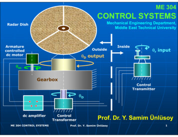
GAIN and PHASE MARGINSNiseNi pp. 638638-641 Gain Margin : Additional gain to makethe system marginally stable at afrequencyqy for which the pphase of theopen loop transfer function passesthrough -180o.Phase Margin : Additional phase angleto make the system marginally stable ata frequency for which the magnitude ofthe open loop transfer function is 0 dB.ME 304 CONTROL SYSTEMSProf. Dr. Y. Samim Ünlüsoy79
GAIN and PHASE MARGINSMaggnitude (dB))50GainGiMargin0-50-100Phase ((deg)-150-90-135-180PhaseM iMargin-225-270-110100101102103Frequency (rad/sec)ME 304 CONTROL SYSTEMSProf. Dr. Y. Samim Ünlüsoy80
BODE PLOT Can youidentify thetransferfunctionapproximatelyif themeasuredmeas redBode diagramis available ?ME 304 CONTROL SYSTEMSProf. Dr. Y. Samim Ünlüsoy81
CONTROL SYSTEMSCONTROL SYSTEMS Mechanical Engineering Department, Middle East Technical University Radar Dish θrinput Armature controlled Outside Inside dc motor θ D output θ m Gearbox Control Transmitter θ D dc amplifier Control Prof Dr Y Samim Ünlüsoy ME 304 CONTROL SYSTEMS Prof.