Transcription
Differential Equations for EngineersLecture Notes forJeffrey R. Chasnov
The Hong Kong University of Science and TechnologyDepartment of MathematicsClear Water Bay, KowloonHong Kongc 2019 by Jeffrey Robert ChasnovCopyright This work is licensed under the Creative Commons Attribution 3.0 Hong Kong License. To view a copy of thislicense, visit http://creativecommons.org/licenses/by/3.0/hk/ or send a letter to Creative Commons, 171 SecondStreet, Suite 300, San Francisco, California, 94105, USA.
PrefaceView the promotional video on YouTubeThese are my lecture notes for my online Coursera course, Differential Equations for Engineers. Ihave divided these notes into chapters called Lectures, with each Lecture corresponding to a video onCoursera. I have also uploaded all my Coursera videos to YouTube, and links are placed at the top ofeach Lecture.There are problems at the end of each lecture chapter and I have tried to choose problems thatexemplify the main idea of the lecture. Students taking a formal university course in differentialequations will usually be assigned many more additional problems, but here I follow the philosophythat less is more. I give enough problems for students to solidify their understanding of the material,but not too many problems that students feel overwhelmed and drop out. I do encourage students toattempt the given problems, but if they get stuck, full solutions can be found in the Appendix.There are also additional problems at the end of coherent sections that are given as practice quizzeson the Coursera platform. Again, students should attempt these quizzes on the platform, but if astudent has trouble obtaining a correct answer, full solutions are also found in the Appendix.Students who take this course are expected to know single-variable differential and integral calculus. Some knowledge of complex numbers, matrix algebra and vector calculus is required for parts ofthis course. Students missing this latter knowledge can find the necessary material in the Appendix.Jeffrey R. ChasnovHong KongJanuary 2019iii
Contents1Introduction to differential equations1Practice quiz: Classify differential equations3IFirst-Order Differential Equations52Euler method93Separable first-order equations114Separable first-order equation: example13Practice quiz: Separable first-order odes155Linear first-order equations176Linear first-order equation: example19Practice quiz: Linear first-order odes217Application: compound interest238Application: terminal velocity259Application: RC circuit27Practice quiz: Applications31IIHomogeneous Linear Differential Equations3310 Euler method for higher-order odes3711 The principle of superposition3912 The Wronskian4113 Homogeneous second-order ode with constant coefficients43Practice quiz: Superposition, the Wronskian, and the characteristic equationv45
CONTENTSvi14 Case 1: Distinct real roots4715 Case 2: Complex-conjugate roots (Part A)4916 Case 2: Complex-conjugate roots (Part B)5117 Case 3: Repeated roots (Part A)5318 Case 3: Repeated roots (Part B)55Practice quiz: Homogeneous equationsIIIInhomogeneous Linear Differential Equations575919 Inhomogeneous second-order ode6320 Inhomogeneous term: Exponential function65Practice quiz: Solving inhomogeneous equations6721 Inhomogeneous term: Sine or cosine (Part A)6922 Inhomogeneous term: Sine or cosine (Part B)7123 Inhomogeneous term: Polynomials73Practice quiz: Particular solutions7524 Resonance7725 Application: RLC circuit7926 Application: Mass on a spring8327 Application: Pendulum8528 Damped resonance87Practice quiz: Applications and resonanceIVThe Laplace Transform and Series Solution Methods899129 Definition of the Laplace transform9530 Laplace transform of a constant-coefficient ode9731 Solution of an initial value problem99Practice quiz: The Laplace transform method10132 The Heaviside step function10333 The Dirac delta function105
CONTENTSvii34 Solution of a discontinuous inhomogeneous term10735 Solution of an impulsive inhomogeneous term109Practice quiz: Discontinuous and impulsive inhomogeneous terms11136 The series solution method11337 Series solution of the Airy’s equation (Part A)11738 Series solution of the Airy’s equation (Part B)121Practice quiz: Series solutionsVSystems of Differential Equations12312539 Systems of linear first-order odes12940 Distinct real eigenvalues13141 Complex-conjugate eigenvalues133Practice quiz: Systems of differential equations13542 Phase portraits13743 Stable and unstable nodes13944 Saddle points14145 Spiral points143Practice quiz: Phase portraits14546 Coupled oscillators14747 Normal modes (eigenvalues)14948 Normal modes (eigenvectors)151Practice quiz: Normal modes153VIPartial Differential Equations15549 Fourier series15950 Fourier sine and cosine series16151 Fourier series: example163Practice quiz: Fourier series52 The diffusion equation165167
CONTENTSviii53 Solution of the diffusion equation (separation of variables)16954 Solution of the diffusion equation (eigenvalues)171Practice quiz: Separable partial differential equations17355 Solution of the diffusion equation (Fourier series)17556 Diffusion equation: example177Practice quiz: The diffusion equationAppendix179180A Complex numbers183B Nondimensionalization185C Matrices and determinants187D Eigenvalues and eigenvectors189E Partial derivatives191F Table of Laplace transforms193G Problem and practice quiz solutions195
Lecture 1Introduction to differential equationsView this lecture on YouTubeA differential equation is an equation for a function containing derivatives of that function. For example, the differential equations for an RLC circuit, a pendulum, and a diffusing dye are given by1d2 qdq R q E0 cos ωt, ( RLC circuit equation)dtCdt2d2 θdθml 2 cl mg sin θ F0 cos ωt, (pendulum equation)dtdt 2 u u 2 u 2 u 2 2 . (diffusion equation) D t x2 y zLThese are second-order differential equations, categorized according to the highest order derivative.The RLC circuit equation (and pendulum equation) is an ordinary differential equation, or ode, andthe diffusion equation is a partial differential equation, or pde. An ode is an equation for a function ofa single variable and a pde for a function of more than one variable. A pde is theoretically equivalentto an infinite number of odes, and numerical solution of nonlinear pdes may require supercomputerresources.The RLC circuit and the diffusion equation are linear and the pendulum equation is nonlinear. Ina linear differential equation, the unknown function and its derivatives appear as a linear polynomial.For instance, the general linear third-order ode, where y y( x ) and primes denote derivatives withrespect to x, is given bya3 ( x )y000 a2 ( x )y00 a1 ( x )y0 a0 ( x )y b( x ),where the a and b coefficients can be any function of x. The pendulum equation is nonlinear becauseof the term sin θ, where θ θ (t) is the unknown function. Making the small angle approximation,sin θ θ, the pendulum equation becomes linear.The simplest type of ode can be solved by integration. For example, a mass such as Newton’sapocryphal apple, falls downward with constant acceleration, and satisfies the differential equationd2 x g.dt2With initial conditions specifying the initial height of the mass x0 and its initial velocity u0 , the solutionobtained by straightforward integration is given by the well-known high school physics equation1x (t) x0 u0 t gt2 .21
2LECTURE 1. INTRODUCTION TO DIFFERENTIAL EQUATIONS
Practice quiz: Classify differentialequations1. By checking all that apply, classify the following differential equation:d2 yd3 y y 2 03dxdxa) first orderb) second orderc) third orderd) ordinarye) partialf ) linearg) nonlinear2. By checking all that apply, classify the following differential equation:1 dξ 2 dξ ξ2dψdξ e ψa) first orderb) second orderc) ordinaryd) partiale) linearf ) nonlinear3
LECTURE 1. INTRODUCTION TO DIFFERENTIAL EQUATIONS43. By checking all that apply, classify the following differential equation: u u 2 u u ν 2 t x xa) first orderb) second orderc) ordinaryd) partiale) linearf ) nonlinear4. By checking all that apply, classify the following differential equation:ad2 xdx b cx 02dtdta) first orderb) second orderc) ordinaryd) partiale) linearf ) nonlinear5. By checking all that apply, classify the following differential equation: 2 u c2 t2 2 u 2 u 2 u 2 2 x2 y z a) first orderb) second orderc) ordinaryd) partiale) linearf ) nonlinearSolutions to the Practice quiz
Week IFirst-Order Differential Equations5
7In this week’s lectures, we discuss first-order differential equations. We begin by explaining theEuler method, which is a simple numerical method for solving an ode. Not all first-order differentialequations have an analytical solution, so it is useful to understand a basic numerical method. Thenthe analytical solution methods for separable and linear equations are explained. We follow the discussion of each theory with some simple examples. Finally, three real-world applications of first-orderequations and their solutions are presented: compound interest, terminal velocity of a falling mass,and the resistor-capacitor electrical circuit.
8
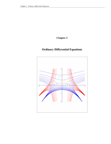
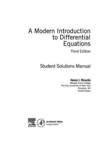
Lecture 2Euler methodView this lecture on YouTubey 1 y0 x f(x0 ,y 0 )y1slope f(x 0,y 0)y0x0x1dy/dx f ( x, y) with initial condition y( x0 ) y0 is integrated to x x1 using the Euler method.Sometimes there is no analytical solution to a first-order differential equation and a numerical solutionmust be sought. The first-order differential equation dy/dx f ( x, y) with initial condition y( x0 ) y0provides the slope f ( x0 , y0 ) of the tangent line to the solution curve y y( x ) at the point ( x0 , y0 ).With a small step size x x1 x0 , the initial condition ( x0 , y0 ) can be marched forward to ( x1 , y1 )along the tangent line using Euler’s method (see figure):y1 y0 x f ( x0 , y0 ).This solution ( x1 , y1 ) then becomes the new initial condition and is marched forward to ( x2 , y2 ) alonga newly determined tangent line with slope given by f ( x1 , y1 ). For small enough x, the numericalsolution converges to the unique solution, when such a solution exists.There are better numerical methods than the Euler method, but the basic principle of marching thesolution forward remains the same.9
LECTURE 2. EULER METHOD10Problems for Lecture 21. The Euler method for solving the differential equation dy/dx f ( x, y) can be rewritten in the formk1 x f ( xn , yn ),y n 1 y n k 1 ,and is called a first-order Runge-Kutta method. More accurate second-order Runge-Kutta methodshave the formk1 x f ( xn , yn ),k2 x f ( xn α x, yn βk1 ),yn 1 yn ak1 bk2 .Some analysis (not shown here) on the second-order Runge-Kutta methods results in the constraintsa b 1,αb βb 1/2.Write down the second-order Runge-Kutta methods corresponding to (i) a b, and (ii) a 0. Thesespecific second-order Runge-Kutta methods are called the modified Euler method and the midpointmethod, respectively.Solutions to the Problems
Lecture 3Separable first-order equationsView this lecture on YouTubeA first-order ode is separable if it can be written in the formg(y)dy f ( x ),dxy ( x0 ) y0 ,where the function g(y) is independent of x and f ( x ) is independent of y. Integration from x0 to xresults inZ xx0g(y( x ))y0 ( x ) dx Z xx0f ( x ) dx.The integral on the left can be transformed by substituting u y( x ), du y0 ( x )dx, and changing thelower and upper limits of integration to y( x0 ) y0 and y( x ) y. Therefore,Z yy0g(u) du Z xx0f ( x ) dx,which can often yield an analytical expression for y y( x ) if the integrals can be done and theresulting algebraic equation can be solved for y.A simpler procedure that yields the same result is to treat dy/dx as a fraction. Multiplying thedifferential equation by dx results directly ing(y) dy f ( x ) dx,which is what we call a separated equation with a function of y times dy on one side, and a functionof x times dx on the other side. This separated equation can then be integrated directly over y and x.11
LECTURE 3. SEPARABLE FIRST-ORDER EQUATIONS12Problems for Lecture 31. Put the following equation in separated form. Do not integrate.a)dyx2 y 4y dxx 4b)dy sec(y)e x y (1 x )dxc)dyxy dx( x 1)(y 1)d)dθ sin θ 0dtSolutions to the Problems
Lecture 4Separable first-order equation: exampleView this lecture on YouTubeExample: Solve y0 y2 sin x 0,y(0) 1.We first manipulate the differential equation to the formdy y2 sin xdxand then treat dy/dx as if it was a fraction to separate variables:dyy2 sin x dx.We then integrate the right side from x equals 0 to x and the left side from y equals 1 to y. We obtainZ y dy1y2 0Integrating, we have 1yor1 Z xsin x dx.xy cos x ,011 cos x 1.ySolving for y, we obtain the solutiony 1.2 cos x13
LECTURE 4. SEPARABLE FIRST-ORDER EQUATION: EXAMPLE14Problems for Lecture 41. Solve the following separable first-order equations. a) dy/dx 4x y, with y(0) 1.b) dx/dt x (1 x ), with x (0) x0 and 0 x0 1.Solutions to the Problems
Practice quiz: Separable first-orderodes1. The solution of y0 a) y( x ) 1 1/2( x 1)29b) y( x ) 1( x 1)29c) y( x ) 1 3/2( x 1)29d) y( x ) 1 2( x 1)29xy with initial value y(1) 0 is given by2. The solution of y2 xy0 0 with initial value y(1) 1 is given bya) y( x ) 11 ln xb) y( x ) 11 2 ln xc) y( x ) 11 ln xd) y( x ) 11 2 ln x3. The solution of y0 (sin x )y 0 with initial value y(π/2) 1 is given bya) y( x ) esin xb) y( x ) ecos xc) y( x ) e1 sin xd) y( x ) e1 cos xSolutions to the Practice quiz15
16LECTURE 4. SEPARABLE FIRST-ORDER EQUATION: EXAMPLE
Lecture 5Linear first-order equationsView this lecture on YouTubeA linear first-order differential equation with initial condition can be written in standard form asdy p ( x ) y g ( x ),dxy ( x0 ) y0 .(5.1)All linear first-order differential equations can be integrated using an integrating factor µ. We multiplythe differential equation by the yet unknown function µ µ( x ) to obtain µ( x ) dy p ( x ) y µ ( x ) g ( x );dxand then require µ( x ) to satisfy the differential equation dydµ( x ) p( x )y [ µ ( x ) y ].dxdx(5.2)The unknown function µ( x ) is called an integrating factor because the resulting differential equation,d[µ( x )y] µ( x ) g( x ), can be directly integrated. Using y( x0 ) y0 and choosing µ( x0 ) 1, we havedxZ xµ ( x ) y y0 µ( x ) g( x ) dx; or after solving for y y( x ),x0y( x ) 1µ( x ) y0 Z xx0 µ( x ) g( x ) dx .(5.3)To determine µ( x ), we expand (5.2) using the product rule to obtain to yieldµdµdydy pµy y µ ;dxdxdxand upon canceling terms, we obtain the differential equationdµ p( x )µ,dxµ( x0 ) 1.This equation is separable and can be easily integrated to obtainµ( x ) exp Zxx0 p( x ) dx .Equations (5.3) and (5.4) together solve the first-order linear equation given by (5.1).17(5.4)
LECTURE 5. LINEAR FIRST-ORDER EQUATIONS18Problems for Lecture 51. Write the following linear equations in standard form.a) xb)dy y sin x;dxdy x y.dx2. Consider the nonlinear differential equation dx/dt x (1 x ). By defining z 1/x, show that theresulting differential equation for z is linear.Solutions to the Problems
Lecture 6Linear first-order equation: exampleView this lecture on YouTubeExample: Solvedy 2y e x , with y(0) 3/4.dxNote that this equation is not separable. With p( x ) 2 and g( x ) e x , we haveµ( x ) expx Z0 2 dx e2x ,andy( x ) e 2x 3 4Z x0 e2x e x dx .Performing the integration, we obtainy( x ) e 2x 3 ( e x 1) ,4which can be simplified to 1y( x ) e x 1 e x .419
LECTURE 6. LINEAR FIRST-ORDER EQUATION: EXAMPLE20Problems for Lecture 61. Solve the following linear odes.a)dy x y,dxb)dy 2x (1 y),dxy(0) 1;y(0) 0.Solutions to the Problems
Practice quiz: Linear first-order odes1. The solution of (1 x2 )y0 2xy 2x with initial value y(0) 0 is given byx1 xxb) y( x ) 1 x2a) y( x ) c) y( x ) x21 xd) y( x ) x21 x22. The solution of x2 y0 1 2xy with initial value y(1) 2 is given bya) y( x ) 1 xxb) y( x ) 1 xx2c) y( x ) 1 x2xd) y( x ) 1 x2x23. The solution of y0 λy a with initial value y(0) 0 and λ 0 is given bya) y( x ) a(1 eλx )b) y( x ) a(1 e λx )a(1 eλx )λad) y( x ) (1 e λx )λc) y( x ) Solutions to the Practice quiz21
22LECTURE 6. LINEAR FIRST-ORDER EQUATION: EXAMPLE
Lecture 7Application: compound interestView this lecture on YouTubeThe compound interest equation arises in many different engineering problems, and we considerit here as it relates to an investment. Let S(t) be the value of the investment at time t, and let r be theannual interest rate compounded after every time interval t. Let k be the annual deposit amount (anegative value indicates a withdrawal), and suppose that a fixed amount is deposited after every timeinterval t. The value of the investment at the time t t is then given byS(t t) S(t) (r t)S(t) k t,(7.1)where at the end of the time interval t, r tS(t) is the amount of interest credited and k t is theamount of money deposited.Rearranging the terms of (7.1) to exhibit what will soon become a derivative, we haveS(t t) S(t) rS(t) k. tThe equation for continuous compounding of interest and continuous deposits is obtained by takingthe limit t 0. The resulting differential equation isdS rS k,dt(7.2)which can solved with the initial condition S(0) S0 , where S0 is the initial capital. The differentialequation is linear and the standard form is dS/dt rS k, so that the integrating factor is given byµ(t) e rt .The solution is thereforeS(t) ert S0 Z t0ke rt dt k S0 ert ert 1 e rt ,rwhere the first term on the right-hand side comes from the initial invested capital, and the secondterm comes from the deposits (or withdrawals). Evidently, compounding results in the exponentialgrowth of an investment.23
24LECTURE 7. APPLICATION: COMPOUND INTERESTProblems for Lecture 71. Suppose a 25 year-old plans to set aside a fixed amount each year until retirement at age 65. Howmuch must he/she save each year to have 1,000,000 at retirement? Assume a 6% annual return on thesaved money compounded continuously. Out of the 1,000,000, approximately how much was saved,and how much was earned on the investment?2. A home buyer can afford to spend no more than 1500 per month on mortgage payments. Supposethat the annual interest rate is 4% and that the term of the mortgage is 30 years. Assume that interest iscompounded continuously and that payments are also made continuously. Determine the maximumamount that this buyer can afford to borrow.Solutions to the Problems
Lecture 8Application: terminal velocityView this lecture on YouTubeUsing Newton’s law, we model a mass m free falling under gravity but with air resistance. We assume that the force of air resistance is proportional to the speed of the mass and opposes the directionof motion. We define the x-axis to point in the upward direction, opposite the force of gravity. Nearthe surface of the Earth, the force of gravity is approximately constant and is given by mg, withg 9.8 m/s2 the usual gravitational acceleration. The force of air resistance is modeled by kv, wherev is the vertical velocity of the mass and k is a positive constant. When the mass is falling, v 0 andthe force of air resistance is positive, pointing upward and opposing the motion. The total force onthe mass is therefore given by F mg kv. With F ma and a dv/dt, we obtain the differentialequationmdv mg kv.dt(8.1)The terminal velocity v of the mass is defined as the asymptotic velocity after air resistance balancesthe gravitational force. When the mass is at terminal velocity, dv/dt 0 so thatv mg.k(8.2)The approach to the terminal velocity of a mass initially at rest is obtained by solving (8.1) with initialcondition v(0) 0. The equation is linear and the standard form is dv/dt (k/m)v g, so that theintegrating factor isµ(t) ekt/m ,and the solution to the differential equation isZ tv(t) e kt/mekt/m ( g) dt0 mg 1 e kt/m . k Therefore, v v 1 e kt/m , and v approaches v as the exponential term decays to zero.25
26LECTURE 8. APPLICATION: TERMINAL VELOCITYProblems for Lecture 81. A male skydiver of mass m 100 kg with his parachute closed may attain a terminal speed of 200km/hr. How long does it take him to attain one-half his terminal speed, and how long to attain 95%?Solutions to the Problems
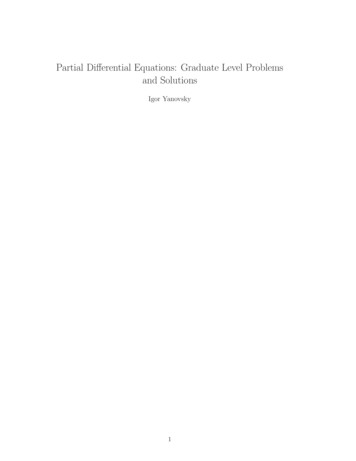
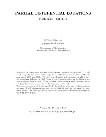
Lecture 9Application: RC circuitView this lecture on YouTubei(a)R(b) CߝRC circuit diagram.Consider a resister R and a capacitor C connected in series as shown in the figure. A battery connectsto this circuit by a switch, stepping up the voltage by E . Initially, there is no charge on the capacitor.When the switch is thrown to a, the battery connects and the capacitor charges. When the switchis thrown to b, the battery disconnects and the capacitor discharges, with energy dissipated in theresister. Here, we determine the voltage drop across the capacitor during charging and discharging.The equations for the voltage drops across a capacitor and a resister are given byVC q/C,VR iR,(9.1)where C is the capacitance and R is the resistance. The charge q and the current i are related byi dq.dt(9.2)Kirchhoff’s voltage law states that the emf E in any closed loop is equal to the sum of the voltagedrops in that loop. Applying Kirchhoff’s voltage law when the switch is thrown to a results inVR VC E .(9.3)Using (9.1) and (9.2), the voltage drop across the resister can be written in terms of the voltage dropacross the capacitor asVR RC27dVC,dt
LECTURE 9. APPLICATION: RC CIRCUIT28and (9.3) can be rewritten to yield the linear first-order differential equation for VC given bydVC VC /RC E /RC,dt(9.4)with initial condition VC (0) 0.The integrating factor for this equation isµ(t) et/RC ,and (9.4) integrates toVC (t) e t/RCZ t0(E /RC )et/RC dt,with solution VC (t) E 1 e t/RC .The voltage starts at zero and rises exponentially to E , with characteristic time scale given by RC.When the switch is thrown to b, application of Kirchhoff’s voltage law results inVR VC 0,with corresponding differential equationdVC VC /RC 0.dtHere, we assume that the capacitance is initially fully charged so that VC (0) E . The solution, then,during the discharge phase is given byVC (t) E e t/RC .The voltage starts at E and decays exponentially to zero, again with characteristic time scale given byRC.
29Problems for Lecture 91. Determine the current in an RC circuit during charging and discharging.Solutions to the Problems
30LECTURE 9. APPLICATION: RC CIRCUIT
Practice quiz: Applications1. Suppose a 25 year-old plans to set aside a fixed amount each year until retirement at age 65.Approximately, how much total must they have set aside to have 1,000,000 at retirement? Assume a10% annual return on the saved money compounded continuously.a) 75,000b) 150,000c) 225,000d) 300,0002. A male skydiver of mass 100 kg with his parachute closed may attain a terminal speed of 200 km/hr.How long does it take him to attain a speed of 150 km/hr?a) 1 sb) 4 sc) 8 sd) 15 s3. An RC circuit consists of a resistor (3000 Ω) and a capacitor (0.001 F), where Ω is the ohm withunits kg · m2 · s 3 · A 2 , F is the Faraday with units s4 · A2 · m 2 · kg 1 , and where kg is kilogram, mis meters, s is seconds, and A is amps. How long does it take for the capacitor to charge to 95% of thebattery voltage?a) 1 sb) 5 sc) 9 sd) 14 sSolutions to the Practice quiz31
32LECTURE 9. APPLICATION: RC CIRCUIT
Week IIHomogeneous Linear DifferentialEquations33
35This week’s lectures are on second-order differential equations. We begin by generalizing the Eulernumerical method to a second-order equation, to show how numerical solutions can be obtained forequations that have no analytical solutions. We then develop two theoretical concepts used for linearequations: the principle of superposition, and the Wronskian. Armed with these concepts, we canthen find analytical solutions to a homogeneous second-order ode with constant coefficients. Wemake use of an exponential ansatz, and convert the differential equation to a quadratic equation calledthe characteristic equation of the ode. The characteristic equation may have real or complex roots andwe discuss the solutions for these different cases.
36
Lecture 10Euler method for higher-order odesView this lecture on YouTubeIn practice, most higher-order odes are solved numerically. For example, consider the general secondorder ode given byẍ f (t, x, ẋ ).Here, we adopt the widely used physics notation ẋ dx/dt and ẍ d2 x/dt2 . The dot notation is usedto represent only time derivatives and can be applied to any dependent variable that is a function oftime.To solve numerically, we convert the second-order ode to a pair of first-order odes. Define u ẋ,and write the first-order system asẋ u,(10.1)u̇ f (t, x, u).(10.2)The first ode, (10.1), gives the slope of the tangent line to the curve x x (t). The second ode, (10.2),gives the slope of the tangent line to the curve u u(t). Beginning at the initial values ( x, u) ( x0 , u0 )at the time t t0 , we move along the tangent lines to determine x1 x (t0 t) and u1 u(t0 t):x1 x0 tu0 ,u1 u0 t f (t0 , x0 , u0 ).The values x1 and u1 at the time t1 t0 t are then used as new initial values to march the solutionforward to time t2 t1 t. When a unique solution of the ode exists, the numerical solutionconverges to this unique solution as t 0.37
38LECTURE 10. EULER METHOD FOR HIGHER-ORDER ODESProblems for Lecture 101. Write the second-order ode, θ̈ θ̇/q sin θ f cos ωt, as a system of two first-order odes.2. Write down the second-order Runge-Kutta modified Euler method (predictor-corrector method) forthe following system of two first-order odes:ẋ f (t, x, y),Solutions to the Problemsẏ g(t, x, y).
Lecture 11The principle of superpositionView this lecture on YouTubeConsider the homogeneous linear second-order ode given byẍ p(t) ẋ q(t) x 0;and suppose that x X1 (t) and x X2 (t) are solutions. We consider a linear combination of X1 andX2 by lettingx c 1 X1 ( t ) c 2 X2 ( t ) ,with c1 and c2 constants. The principle of superposition states that x is also a solution to the homogeneousode. To prove this, we compute ẍ p ẋ qx c1 Ẍ1 c2 Ẍ2 p c1 Ẋ1 c2 Ẋ2 q (c1 X1 c2 X2 ) c1 Ẍ1 p Ẋ1 qX1 c2 Ẍ2 p Ẋ2 qX2 c1 0 c2 0 0,since X1 and X2 were assumed to be solutions of the homogeneous ode. We have therefore shown thatany linear combination of solutions to the homogeneous linear second-order ode is also a solution.39
40LECTURE 11. THE PRINCIPLE OF SUPERPOSITIONProblems for Lecture 111. Consider the inhomogeneous linear second-order ode given byẍ p(t) ẋ q(t) x g(t);and suppose that x xh (t) is a solution of the homogeneous equation and x x p (t) is a solutionof the inhomogeneous equation. Prove that x xh (t) x p (t) is a solution of the inhomogeneousequation.Solutions to the Problems
Lecture 12The WronskianView this lecture on YouTubeSuppose that we have determined that x X1 (t) and x X2 (t) are solutions toẍ p(t) ẋ q(t) x 0,and that we now attempt to write the general solution to the ode asx c 1 X1 ( t ) c 2 X2 ( t ) .We must then ask whether this general solution can satisfy the two initial conditions given byx ( t0 ) x0 ,ẋ (t0 ) u0 .Applying these initial conditions to our proposed general solution, we obtainc 1 X1 ( t 0 ) c 2 X2 ( t 0 ) x 0 ,c1 Ẋ1 (t0 ) c2 Ẋ2 (t0 ) u0 ,which is a system of two linear equations for c1 and c2 . A unique solution exists providedW X1 ( t 0 )X2 ( t 0 )Ẋ1 (t0 )Ẋ2 (t0 ) X1 (t0 ) Ẋ2 (t0 ) Ẋ1 (t0 ) X2 (t0 ) 6 0,where the determinant given by W is called the Wronskian.For example, with ω 6 0, the two solutions X1 (t) cos ωt and X2 (t) sin ωt have a nonzeroWronskian for all t sinceW (cos ωt) (ω cos ωt) ( ω sin ωt) (sin ωt) ω.When the Wronskian is not equal to zero, we say that the two solutions X1 (t) and X2 (t) are linearlyindependent. The concept of linear independence is borrowed from linear algebra, and indeed, theset of all functions that satisfy a second-order linear homogeneous ode can be shown to form a twodimensional vector space.41
42LECTURE 12. THE WRONSKIANProblems for Lecture 121. Show that X1 (t) exp (αt) and X2 (t) exp ( βt) have a nonzero Wronskian for all t providedα 6 β.Solutions to the Problems
Lecture 13Homogeneous second-order ode withconstant coefficientsView this lecture on YouTubeWe now study solutions of the homogeneous constant-coefficient ode, written asa ẍ b ẋ cx 0,with a, b, and c constants. Our solution method finds two linearly independent solutions, multiplieseach of these solutions by a constant, and adds them. The two free constants are then determinedfrom initial values on x and ẋ.Because of the differential properties of the exponential function, a natural ansatz, or educatedguess, for the form of the solution is x ert , where r is a constant to be determined. Successivedifferentiation results in ẋ rert and ẍ r2 ert , and substitution into the ode yieldsar2 ert brert cert 0.Our choice of exponential function is now rewarded by the explicit cancelation of ert . The result is aquadratic equation for the unknown constant r:ar2 br c 0.Our ansatz has thus converted a differential equation for x into an algebraic equation for r. Thisalgebraic equation is called the characteristic equation of the ode. Using the quadratic formula, the twosolutions of the characteristic equ
These are my lecture notes for my online Coursera course,Differential Equations for Engineers. I have divided these notes into chapters called Lectures, with each Lecture corresponding to a video on Coursera. I have also uploaded all my Coursera videos to