Transcription
MAT 169: Calculus III with Analytic GeometryJames V. LambersApril 12, 2012
2
Contents1 Sequences and Series1.1 Introduction . . . . . . . . . . . . . . . . . . . . . . .1.1.1 Sequences and Series . . . . . . . . . . . . . .1.1.2 Vectors and the Geometry of Space . . . . . .1.1.3 Parametric Equations and Polar Coordinates1.2 Review of Calculus . . . . . . . . . . . . . . . . . . .1.2.1 Limits . . . . . . . . . . . . . . . . . . . . . .1.2.2 Continuity . . . . . . . . . . . . . . . . . . .1.2.3 Derivatives . . . . . . . . . . . . . . . . . . .1.2.4 Riemann Sums and the Definite Integral . . .1.2.5 Extreme Values . . . . . . . . . . . . . . . . .1.2.6 The Mean Value Theorem . . . . . . . . . . .1.2.7 The Mean Value Theorem for Integrals . . .1.3 Taylor’s Theorem . . . . . . . . . . . . . . . . . . . .1.4 Sequences . . . . . . . . . . . . . . . . . . . . . . . .1.4.1 What is a Sequence? . . . . . . . . . . . . . .1.4.2 Why Do We Need Sequences? . . . . . . . . .1.4.3 Recognizing Sequences . . . . . . . . . . . . .1.4.4 Limits of Sequences . . . . . . . . . . . . . .1.4.5 Relation to Limits of Functions . . . . . . . .1.4.6 Testing Convergence of Sequences . . . . . .1.4.7 Alternating Sequences . . . . . . . . . . . . .1.4.8 Growth Rates of Functions . . . . . . . . . .1.4.9 Geometric Sequences . . . . . . . . . . . . . .1.4.10 Recursively Defined Sequences . . . . . . . .1.4.11 Bounded and Monotonic Sequences . . . . . .1.4.12 Summary . . . . . . . . . . . . . . . . . . . .1.5 Series . . . . . . . . . . . . . . . . . . . . . . . . . .1.5.1 What is a Series? . . . . . . . . . . . . . . . 353737
4CONTENTS1.5.2 Why Do We Need Series? . . . . . . . . . . . .1.5.3 Geometric Series . . . . . . . . . . . . . . . . .1.5.4 Telescoping Series . . . . . . . . . . . . . . . .1.5.5 Harmonic Series . . . . . . . . . . . . . . . . .1.5.6 Basic Convergence Tests . . . . . . . . . . . . .1.5.7 Summary . . . . . . . . . . . . . . . . . . . . .1.6 Convergence Tests . . . . . . . . . . . . . . . . . . . .1.6.1 The Integral Test . . . . . . . . . . . . . . . . .1.6.2 The Comparison Test . . . . . . . . . . . . . .1.7 Other Convergence Tests . . . . . . . . . . . . . . . . .1.7.1 The Alternating Series Test . . . . . . . . . . .1.7.2 Estimating Error in Alternating Series . . . . .1.7.3 Absolute Convergence . . . . . . . . . . . . . .1.7.4 The Ratio Test . . . . . . . . . . . . . . . . . .1.7.5 The Root Test . . . . . . . . . . . . . . . . . .1.7.6 Summary . . . . . . . . . . . . . . . . . . . . .1.8 Power Series . . . . . . . . . . . . . . . . . . . . . . . .1.8.1 What is a Power Series? . . . . . . . . . . . . .1.8.2 Convergence of Power Series . . . . . . . . . .1.8.3 The Radius of Convergence . . . . . . . . . . .1.8.4 Representing Functions as Power Series . . . .1.8.5 Differentiation and Integration of Power Series1.8.6 Summary . . . . . . . . . . . . . . . . . . . . .1.9 Taylor and Maclaurin Series . . . . . . . . . . . . . . .1.9.1 Summary . . . . . . . . . . . . . . . . . . . . .1.10 Review . . . . . . . . . . . . . . . . . . . . . . . . . . .2 Vectors and the Geometry of Space2.1 Three-Dimensional Coordinate Systems .2.1.1 Points in Three-Dimensional Space2.1.2 Planes in Three-Dimensional Space2.1.3 Plotting Points in xyz-space . . . .2.1.4 The Distance Formula . . . . . . .2.1.5 Equations of Surfaces . . . . . . .2.1.6 Summary . . . . . . . . . . . . . .2.2 Vectors . . . . . . . . . . . . . . . . . . .2.2.1 Combining Vectors . . . . . . . . .2.2.2 Components . . . . . . . . . . . .2.2.3 Summary . . . . . . . . . . . . . .2.3 The Dot Product . . . . . . . . . . . . . 082.8787878889899092939495102103
CONTENTS2.42.52.62.3.1 Properties . . . . . . . . . . . . .2.3.2 Orthogonality . . . . . . . . . . .2.3.3 Projections . . . . . . . . . . . .2.3.4 Summary . . . . . . . . . . . . .The Cross Product . . . . . . . . . . . .2.4.1 Parallel Vectors . . . . . . . . . .2.4.2 Properties . . . . . . . . . . . . .2.4.3 Areas . . . . . . . . . . . . . . .2.4.4 Volumes . . . . . . . . . . . . . .2.4.5 Summary . . . . . . . . . . . . .Equations of Lines and Planes . . . . . .2.5.1 Equations of Lines . . . . . . . .2.5.2 Systems of Linear Equations . .2.5.3 Equations of Planes . . . . . . .2.5.4 Intersecting Planes . . . . . . . .2.5.5 Distance from a Point to a Plane2.5.6 Summary . . . . . . . . . . . . .Review . . . . . . . . . . . . . . . . . . 01311333 Parametric Curves and Polar Coordinates1433.1 Parametric Curves . . . . . . . . . . . . . . . . . . . . . . . . 1433.1.1 Summary . . . . . . . . . . . . . . . . . . . . . . . . . 1473.2 Calculus with Parametric Curves . . . . . . . . . . . . . . . . 1483.2.1 Arc Length . . . . . . . . . . . . . . . . . . . . . . . . 1483.2.2 Arc Length of Parametrically Defined Curves . . . . . 1513.2.3 Tangents of Parametric Curves . . . . . . . . . . . . . 1553.2.4 Areas Under Parametric Curves . . . . . . . . . . . . 1613.2.5 Summary . . . . . . . . . . . . . . . . . . . . . . . . . 1643.3 Polar Coordinates . . . . . . . . . . . . . . . . . . . . . . . . 1653.3.1 Conversion Between Cartesian and Polar Coordinates 1663.3.2 Polar Equations . . . . . . . . . . . . . . . . . . . . . 1683.3.3 Tangents to Polar Curves . . . . . . . . . . . . . . . . 1713.3.4 Summary . . . . . . . . . . . . . . . . . . . . . . . . . 1743.4 Areas and Lengths in Polar Coordinates . . . . . . . . . . . . 1743.4.1 Area . . . . . . . . . . . . . . . . . . . . . . . . . . . . 1743.4.2 Arc Length . . . . . . . . . . . . . . . . . . . . . . . . 1793.4.3 Summary . . . . . . . . . . . . . . . . . . . . . . . . . 1803.5 Review . . . . . . . . . . . . . . . . . . . . . . . . . . . . . . . 181Index184
6CONTENTS
Chapter 1Sequences and Series1.1IntroductionThis course is the third course in the calculus sequence, following MAT167 and MAT 168. Its purpose is to prepare students for more advancedmathematics courses, particularly those pertaining to multivariable calculus(MAT 280) and numerical analysis (MAT 460 and 461). The course willfocus on three main areas, which we briefly discuss here.1.1.1Sequences and SeriesNearly all students have had to use a scientific calculator. Consider the following: how does a calculator efficiently evaluate many of its functions, suchas sin, cos or exp, when its hardware is only able to perform the four basicarithmetic operations, addition, subtraction, multiplication and division?The answer stems from the fact that it is generally not possible to evaluate such functions exactly; rather, one has to settle for an approximation.However, this is no problem, because a calculator or computer can only represent real numbers to limited accuracy anyway. To approximate a givenfunction in a manner that is suitable for a calculator, we use infinite series,which is a sum of infinitely many terms. For example, we can write X 111exp x 1 x x2 x3 · · · xk .26k!k 0The last term in the above equation uses sigma notation to express a sum ofinfinitely many terms in a concise way, when those terms can be describedby a pattern. The above series is called a power series because each of its7
8CHAPTER 1. SEQUENCES AND SERIESterms features a power of x. When we study infinite series, we will considerimportant questions such as When does an infinite series sum, or converge, to a finite number?We will see that in many cases, a sum of infinitely many terms doesnot converge at all, but rather continues growing, or diverging. Forexample, consider the two series X1,nn 1 Xn 11.n1.01Although the individual terms in the series may not differ by verymuch, especially for larger values of n, the first series does not converge, while the second one does. If we truncate a series after a given number of terms, how well does thesum of the retained terms approximate the sum of the entire series?This is particularly important when using series to evaluate functionssuch as those implemented in scientific calculators. For example, suppose we take the abovementioned series for exp x and compute onlythe first 20 terms. If x 0.1, then the result is correct to at least 16significant digits. However, if x 10, then we only obtain two correctdigits.1.1.2Vectors and the Geometry of SpaceNext, we will become acquainted with three-dimensional space, in orderto prepare you for later coursework in multivariable calculus. Our basictools will be vectors, which can be used to represent either a position ordirection in space. For example, if we represent three-dimensional spaceusing Cartesian coordinates x, y and z, then the origin is the point withcoordinates x 0, y 0 and z 0, typically denoted by the ordered triple(0, 0, 0). Then, the point in space (1, 0, 2) has coordinates x 1, y 0 andz 2, meaning that it is located 1 unit from the origin along the positivex-axis, 0 units from the origin along the y-axis, and 2 units from the originalong the negative z-axis. This is illustrated in Figure 1.1. We will usevectors to facilitate the description of, and operations on, lines and planes.This is particularly useful in computer graphics. Consider the problem ofrendering a two-dimensional image, say for a frame in a film, of a collectionof three-dimensional objects. To what point in 2-D space does any givenpoint in 3-D space correspond? This question is answered by computing
1.1. INTRODUCTION9Figure 1.1: The origin in three-dimensional space, and the point (1, 0, 2).the projection of points in 3-D space onto a given plane in 2-D space thatcorresponds to the “screen”. We will learn about an operation called thedot product that is used to compute projections. Another operation, calledthe cross product, is very useful for describing planes.1.1.3Parametric Equations and Polar CoordinatesFinally, will study curves and surfaces in space. Often, it is necessary todescribe the position of an object as a function of time. Therefore, wewill study curves that are described by parametric equations, where theparameter is usually time. For example, in combat, the military needs totrack the position of enemy projectiles over time. Using radar data, theycan then construct parametric equations for the projectile’s position in 3-Dspace, and then differentiate the equations with respect to time in order toestimate its velocity and then its trajectory, so that it can be intercepted.While we will work with Cartesian coordinates x, y and z for most of thecourse, we will find that it is often useful to represent curves or functionsin the xy-plane using polar coordinates r and θ, where r represents distancefrom the origin, and θ represents the angle that the point makes with theorigin and the positive x-axis. For example, the point x 0, y 1, which is
10CHAPTER 1. SEQUENCES AND SERIES1 unit from the origin and makes a 90-degree angle with the origin and thepositive x-axis, has polar coordinates (1, π/2). Certain curves are far moreeasily described using polar coordinates. To see this, consider the equationsr sin 2t,(x2 y 2 )3/2 2xy.These two equations describe the same curve, which resembles a four-leafclover. We will learn how to compute areas of regions enclosed by parametric curves, and lengths of parametric curves, that are expressed in eitherCartesian or polar coordinates.1.2Review of CalculusWe now review some basic concepts from the first two calculus courses beforewe begin our study of the third. Recall that these two courses focused onthe following fundamental problems: computing the instantaneous rate of change of one quantity with respect to another, which is a derivative, and computing the total change in a function over some portion of itsdomain, which is a definite integral.1.2.1LimitsThe basic problems of differential and integral calculus described in the previous paragraph can be solved by computing a sequence of approximationsto the desired quantity and then determining what value, if any, the sequence of approximations approaches. This value is called a limit of thesequence. As a sequence is a function, we begin by defining, precisely, theconcept of the limit of a function.Definition We writelim f (x) Lx aif for any open interval I1 containing L, there is some open interval I2containing a such that f (x) I1 whenever x I2 , and x 6 a. We say thatL is the limit of f (x) as x approaches a.We writelim f (x) Lx a if, for any open interval I1 containing L, there is an open interval I2 of theform (c, a), where c a, such that f (x) I1 whenever x I2 . We say that
1.2. REVIEW OF CALCULUS11L is the limit of f (x) as x approaches a from the left, or the left-handlimit of f (x) as x approaches a.Similarly, we writelim f (x) Lx a if, for any open interval I1 containing L, there is an open interval I2 of theform (a, c), where c a, such that f (x) I1 whenever x I2 . We saythat L is the limit of f (x) as x approaches a from the right, or theright-hand limit of f (x) as x approaches a.We can make the definition of a limit a little more concrete by imposingsizes on the intervals I1 and I2 , as long as the interval I1 can still be ofarbitrary size. It can be shown that the following definition is equivalent tothe previous one.Definition We writelim f (x) Lx aif, for any 0, there exists a number δ 0 such that f (x) L whenever 0 x a δ.Similar definitions can be given for the left-hand and right-hand limits.Note that in either definition, the point x a is specifically excludedfrom consideration when requiring that f (x) be close to L whenever x isclose to a. This is because the concept of a limit is only intended to describethe behavior of f (x) near x a, as opposed to its behavior at x a. Laterin this section we discuss the case where the two distinct behaviors coincide.1.2.2ContinuityIn many cases, the limit of a function f (x) as x approached a could beobtained by simply computing f (a). Intuitively, this indicates that f has tohave a graph that is one continuous curve, because any “break” or “jump”in the graph at x a is caused by f approaching one value as x approachesa, only to actually assume a different value at a. This leads to the followingprecise definition of what it means for a function to be continuous at a givenpoint.Definition (Continuity) We say that a function f is continuous at a iflim f (x) f (a).x aWe also say that f (x) has the Direct Subsitution Property at x a.
12CHAPTER 1. SEQUENCES AND SERIESWe say that a function f is continuous from the right at a iflim f (x) f (a).x a Similarly, we say that f is continuous from the left at a iflim f (x) f (a).x a The preceding definition describes continuity at a single point. In describing where a function is continuous, the concept of continuity over aninterval is useful, so we define this concept as well.Definition (Continuity on an Interval) We say that a function f is continuous on the interval (a, b) if f is continuous at every point in (a, b).Similarly, we say that f is continuous on1. [a, b) if f is continuous on (a, b), and continuous from the right at a.2. (a, b] if f is continuous on (a, b), and continuous from the left at b.3. [a, b] if f is continuous on (a, b), continuous from the right at a, andcontinuous from the left at b.1.2.3DerivativesThe basic problem of differential calculus is computing the instantaneousrate of change of one quantity y with respect to another quantity x. Forexample, y may represent the position of an object and x may representtime, in which case the instantaneous rate of change of y with respect to xis interpreted as the velocity of the object.When the two quantities x and y are related by an equation of the formy f (x), it is certainly convenient to describe the rate of change of y withrespect to x in terms of the function f . Because the instantaneous rateof change is so commonplace, it is practical to assign a concise name andnotation to it, which we do now.Definition (Derivative) The derivative of a function f (x) at x a, denoted by f 0 (a), isf (a h) f (a)f 0 (a) lim,h 0hprovided that the above limit exists. When this limit exists, we say that f isdifferentiable at a.
1.2. REVIEW OF CALCULUS13Remark Given a function f (x) that is differentiable at x a, the followingnumbers are all equal: the derivative of f at x a, f 0 (a), the slope of the tangent line of f at the point (a, f (a)), and the instantaneous rate of change of y f (x) with respect to x atx a.This can be seen from the fact that all three numbers are defined in thesame way. 21.2.4Riemann Sums and the Definite IntegralThere are many cases in which some quantity is defined to be the productof two other quantities. For example, a rectangle of width w has uniformheight h, and the area A of the rectangle is given by the formula A wh. Unfortunately, in many applications, we cannot necessarily assume thatcertain quantities such as height are constant, and therefore formulas suchas A wh cannot be used directly. However, they can be used indirectly tosolve more general problems by employing the notation known as integralcalculus.Suppose we wish to compute the area of a shape that is not a rectangle.To simplify the discussion, we assume that the shape is bounded by thevertical lines x a and x b, the x-axis, and the curve defined by somecontinuous function y f (x), where f (x) 0 for a x b. Then, we canapproximate this shape by n rectangles that have width x (b a)/nand height f (xi ), where xi a i x, for i 0, . . . , n. We obtain theapproximationnXA An f (xi ) x.i 1Intuitively, we can conclude that as n , the approximate area An willconverge to the exact area of the given region. This can be seen by observingthat as n increases, the n rectangles defined above comprise a more accurateapproximation of the region.More generally, suppose that for each n 1, 2, . . ., we define the quantityRn by choosing points a x0 x1 · · · xn b, and computing the sumRn nXi 1f (x i ) xi , xi xi xi 1 ,xi 1 x i xi .
14CHAPTER 1. SEQUENCES AND SERIESThe sum that defines Rn is known as a Riemann sum. Note that the interval[a, b] need not be divided into subintervals of equal width, and that f (x) canbe evaluated at arbitrary points belonging to each subinterval.If f (x) 0 on [a, b], then Rn converges to the area under the curvey f (x) as n , provided that the widths of all of the subintervals[xi 1 , xi ], for i 1, . . . , n, approach zero. This behavior is ensured if werequire thatlim δ(n) 0,n whereδ(n) max xi .1 i nThis condition is necessary because if it does not hold, then, as n , theregion formed by the n rectangles will not converge to the region whose areawe wish to compute. If f assumes negative values on [a, b], then, under thesame conditions on the widths of the subintervals, Rn converges to the netarea between the graph of f and the x-axis, where area below the x-axis iscounted negatively.We define the definite integral of f (x) from a to b byZbf (x) dx lim Rn ,an where the sequence of Riemann sums {Rn } n 1 is defined so that δ(n) 0 as n , as in the previous discussion. The function f (x) is calledthe integrand, and the values a and b are the lower and upper limits ofintegration, respectively. The process of computing an integral is calledintegration.1.2.5Extreme ValuesIn many applications, it is necessary to determine where a given functionattains its minimum or maximum value. For example, a business wishesto maximize profit, so it can construct a function that relates its profit tovariables such as payroll or maintenance costs. We now consider the basicproblem of finding a maximum or minimum value of a general function f (x)that depends on a single independent variable x. First, we must preciselydefine what it means for a function to have a maximum or minimum value.Definition (Absolute extrema) A function f has a absolute maximum orglobal maximum at c if f (c) f (x) for all x in the domain of f . Thenumber f (c) is called the maximum value of f on its domain. Similarly, fhas a absolute minimum or global minimum at c if f (c) f (x) for all
1.2. REVIEW OF CALCULUS15x in the domain of f . The number f (c) is then called the minimum valueof f on its domain. The maximum and minimum values of f are called theextreme values of f , and the absolute maximum and minimum are eachcalled an extremum of f .Before computing the maximum or minimum value of a function, it is naturalto ask whether it is possible to determine in advance whether a functioneven has a maximum or minimum, so that effort is not wasted in trying tosolve a problem that has no solution. The following result is very helpful inanswering this question.Theorem (Extreme Value Theorem) If f is continuous on [a, b], then f hasan absolute maximum and an absolute minimum on [a, b].Now that we can easily determine whether a function has a maximum orminimum on a closed interval [a, b], we can develop an method for actuallyfinding them. It turns out that it is easier to find points at which f attainsa maximum or minimum value in a “local” sense, rather than a “global”sense. In other words, we can best find the absolute maximum or minimumof f by finding points at which f achieves a maximum or minimum withrespect to “nearby” points, and then determine which of these points is theabsolute maximum or minimum. The following definition makes this notionprecise.Definition (Local extrema) A function f has a local maximum at c iff (c) f (x) for all x in an open interval containing c. Similarly, f has alocal minimum at c if f (c) f (x) for all x in an open interval containingc. A local maximum or local minimum is also called a local extremum.At each point at which f has a local maximum, the function either hasa horizontal tangent line, or no tangent line due to not being differentiable.It turns out that this is true in general, and a similar statement applies tolocal minima. To state the formal result, we first introduce the followingdefinition, which will also be useful when describing a method for findinglocal extrema.Definition(Critical Number) A number c in the domain of a function f isa critical number of f if f 0 (c) 0 or f 0 (c) does not exist.The following result describes the relationship between critical numbers andlocal extrema.Theorem (Fermat’s Theorem) If f has a local minimum or local maximum
16CHAPTER 1. SEQUENCES AND SERIESat c, then c is a critical number of f ; that is, either f 0 (c) 0 or f 0 (c) doesnot exist.This theorem suggests that the maximum or minimum value of a functionf (x) can be found by solving the equation f 0 (x) 0.1.2.6The Mean Value TheoremWhile the derivative describes the behavior of a function at a point, we oftenneed to understand how the derivative influences a function’s behavior on aninterval. It is often necessary to approximate a function f (x) by a functiong(x) using knowledge of f (x) and its derivatives at various points. It istherefore natural to ask how well g(x) approximates f (x) away from thesepoints.The following result, a consequence of Fermat’s Theorem, gives limitedinsight into the relationship between the behavior of a function on an intervaland the value of its derivative at a point.Theorem (Rolle’s Theorem) If f is continuous on a closed interval [a, b]and is differentiable on the open interval (a, b), and if f (a) f (b), thenf 0 (c) 0 for some number c in (a, b).By applying Rolle’s Theorem to a function f , then to its derivative f 0 , itssecond derivative f 00 , and so on, we obtain the following more general result,which will be useful in analyzing the accuracy of methods for approximatingfunctions by polynomials.Theorem (Generalized Rolle’s Theorem) Let x0 , x1 , x2 , . . . , xn be distinctpoints in an interval [a, b]. If f is n times differentiable on (a, b), and iff (xi ) 0 for i 0, 1, 2, . . . , n, then f (n) (c) 0 for some number c in (a, b).A more fundamental consequence of Rolle’s Theorem is the Mean ValueTheorem itself, which we now state.Theorem (Mean Value Theorem) If f is continuous on a closed interval[a, b] and is differentiable on the open interval (a, b), thenf (b) f (a) f 0 (c)b afor some number c in (a, b).Remark The expressionf (b) f (a)b a
1.2. REVIEW OF CALCULUS17is the slope of the secant line passing through the points (a, f (a)) and(b, f (b)). The Mean Value Theorem therefore states that under the givenassumptions, the slope of this secant line is equal to the slope of the tangentline of f at the point (c, f (c)), where c (a, b). 2The Mean Value Theorem has the following practical interpretation: theaverage rate of change of y f (x) with respect to x on an interval [a, b] isequal to the instantaneous rate of change y with respect to x at some pointin (a, b).1.2.7The Mean Value Theorem for IntegralsSuppose that f (x) is a continuous function on an interval [a, b]. Then, by theFundamental Theorem of Calculus, f (x) has an antiderivative F (x) definedon [a, b] such that F 0 (x) f (x). If we apply the Mean Value Theorem toF (x), we obtain the following relationship between the integral of f over[a, b] and the value of f at a point in (a, b).Theorem (Mean Value Theorem for Integrals) If f is continuous on [a, b],thenZ bf (x) dx f (c)(b a)afor some c in (a, b).In other words, f assumes its average value over [a, b], defined byfave1 b aZbf (x) dx,aat some point in [a, b], just as the Mean Value Theorem states that thederivative of a function assumes its average value over an interval at somepoint in the interval.The Mean Value Theorem for Integrals is also a special case of the following more general result.Theorem (Weighted Mean Value Theorem for Integrals) If f is continuouson [a, b], and g is a function that is integrable on [a, b] and does not changesign on [a, b], thenZbZf (x)g(x) dx f (c)afor some c in (a, b).bg(x) dxa
18CHAPTER 1. SEQUENCES AND SERIESIn the case where g(x) is a function that is easy to antidifferentiate andf (x) is not, this theorem can be used to obtain an estimate of the integralof f (x)g(x) over an interval.Example Let f (x) be continuous on the interval [a, b]. Then, for any x [a, b], by the Weighted Mean Value Theorem for Integrals, we haveZxZx(s a) ds f (c)f (s)(s a) ds f (c)aa(s a)22x f (c)a(x a)2,2where a c x. It is important to note that we can apply the WeightedMean Value Theorem because the function g(x) (x a) does not changesign on [a, b]. 21.3Taylor’s TheoremIn many cases, it is useful to approximate a given function f (x) by a polynomial, because one can work much more easily with polynomials than withother types of functions. As such, it is necessary to have some insight intothe accuracy of such an approximation. The following theorem, which is aconsequence of the Weighted Mean Value Theorem for Integrals, providesthis insight.Theorem (Taylor’s Theorem) Let f be n times continuously differentiableon an interval [a, b], and suppose that f (n 1) exists on [a, b]. Let x0 [a, b].Then, for any point x [a, b],f (x) Pn (x) Rn (x),wherePn (x) nXf (j) (x0 )j!j 0(x x0 )j1f (n) (x0 ) f (x0 ) f 0 (x0 )(x x0 ) f 00 (x0 )(x x0 )2 · · · (x x0 )n2n!andZxRn (x) x0f (n 1) (s)f (n 1) (ξ(x))(x s)n ds (x x0 )n 1 ,n!(n 1)!where ξ(x) is between x0 and x.
1.3. TAYLOR’S THEOREM19The polynomial Pn (x) is the nth Taylor polynomial of f with center x0 ,and the expression Rn (x) is called the Taylor remainder of Pn (x). Whenthe center x0 is zero, the nth Taylor polynomial is also known as the nthMaclaurin polynomial.The final form of the remainder is obtained by applying the Mean ValueTheorem for Integrals to the integral form. As Pn (x) can be used to approximate f (x), the remainder Rn (x) is also referred to as the truncationerror of Pn (x). The accuracy of the approximation on an interval can beanalyzed by using techniques for finding the extreme values of functions tobound the (n 1)-st derivative on the interval.Because approximation of functions by polynomials is employed in thedevelopment and analysis of many techniques in numerical analysis, theusefulness of Taylor’s Theorem cannot be overstated. In fact, it can be saidthat Taylor’s Theorem is the Fundamental Theorem of Numerical Analysis,just as the theorem describing inverse relationship between derivatives andintegrals is called the Fundamental Theorem of Calculus.We conclude our discussion of Taylor’s Theorem with some examples thatillustrate how the nth-degree Taylor polynomial Pn (x) and the remainderRn (x) can be computed for a given function f (x).Example If we set n 1 in Taylor’s Theorem, then we havef (x) P1 (x) R1 (x)whereP1 (x) f (x0 ) f 0 (x0 )(x x0 ).This polynomial is a linear function that describes the tangent line to thegraph of f at the point (x0 , f (x0 )).If we set n 0 in the theorem, then we obtainf (x) P0 (x) R0 (x),whereP0 (x) f (x0 )andR0 (x) f 0 (ξ(x))(x x0 ),where ξ(x) lies between x0 and x. If we use the integral form of the remainder,Z x (n 1)f(s)Rn (x) (x s)n ds,n!x0
20CHAPTER 1. SEQUENCES AND SERIESthen we haveZxf (x) f (x0 ) f 0 (s) ds,x0which is equivalent to the Total Change Theorem and part of the Fundamental Theo
1.1.2 Vectors and the Geometry of Space Next, we will become acquainted with three-dimensional space, in order to prepare you for later coursework in multivariable calculus. Our basic tools will be vectors, which can be used to represent either a position or direction in sp