Transcription
IntroductionRandom matrix theoryEstimating correlationsComparison with BarraRandom Matrix TheoryandCovariance EstimationJim GatheralNew York, October 3, 2008ConclusionAppendix
IntroductionRandom matrix theoryEstimating correlationsComparison with BarraConclusionAppendixMotivationSophisticated optimal liquidation portfolio algorithms that balancerisk against impact cost involve inverting the covariance matrix.Eigenvalues of the covariance matrix that are small (or even zero)correspond to portfolios of stocks that have nonzero returns butextremely low or vanishing risk; such portfolios are invariablyrelated to estimation errors resulting from insuffient data. One ofthe approaches used to eliminate the problem of small eigenvaluesin the estimated covariance matrix is the so-called random matrixtechnique. We would like to understand:the basis of random matrix theory. (RMT)how to apply RMT to the estimation of covariance matrices.whether the resulting covariance matrix performs better than(for example) the Barra covariance matrix.
IntroductionRandom matrix theoryEstimating correlationsComparison with BarraOutline1Random matrix theoryRandom matrix examplesWigner’s semicircle lawThe Marčenko-Pastur densityThe Tracy-Widom lawImpact of fat tails2Estimating correlationsUncertainty in correlation estimates.Example with SPX stocksA recipe for filtering the sample correlation matrix3Comparison with BarraComparison of eigenvectorsThe minimum variance portfolioComparison of weightsIn-sample and out-of-sample performance45ConclusionsAppendix with a sketch of Wigner’s original proofConclusionAppendix
IntroductionRandom matrix theoryEstimating correlationsComparison with BarraConclusionAppendixExample 1: Normal random symmetric matrixGenerate a 5,000 x 5,000 random symmetric matrix withentries aij N(0, 1).Compute eigenvalues.Draw a histogram.Here’s some R-code to generate a symmetric random matrix whoseoff-diagonal elements have variance 1/N:n - 5000;m - array(rnorm(n 2),c(n,n));m2 - (m t(m))/sqrt(2*n);# Make m symmetriclambda - eigen(m2, symmetric T, only.values T);e - lambda values;hist(e,breaks seq(-2.01,2.01,.02),main NA, xlab "Eigenvalues",freq F)
IntroductionRandom matrix theoryEstimating correlationsComparison with BarraExample 1: continued0.20.10.0Density0.30.4Here’s the result: 2 10Eigenvalues12ConclusionAppendix
IntroductionRandom matrix theoryEstimating correlationsComparison with BarraConclusionAppendixExample 2: Uniform random symmetric matrixGenerate a 5,000 x 5,000 random symmetric matrix withentries aij Uniform(0, 1).Compute eigenvalues.Draw a histogram.Here’s some R-code again:n - 5000;mu - array(runif(n 2),c(n,n));mu2 -sqrt(12)*(mu t(mu)-1)/sqrt(2*n);lambdau - eigen(mu2, symmetric T, only.values T);eu - lambdau values;hist(eu,breaks seq(-2.05,2.05,.02),main NA,xlab "Eigenvalueeu - lambdau values;histeu -hist(eu,breaks seq(-2.01,2.01,0.02),main NA, xlab "Eigenvalues",freq F)
IntroductionRandom matrix theoryEstimating correlationsComparison with BarraExample 2: continued0.20.10.0Density0.30.4Here’s the result: 2 10Eigenvalues12ConclusionAppendix
IntroductionRandom matrix theoryEstimating correlationsComparison with BarraConclusionWhat do we see?We note a striking pattern: the density of eigenvalues is asemicircle!Appendix
IntroductionRandom matrix theoryEstimating correlationsComparison with BarraConclusionWigner’s semicircle lawConsider an N N matrix à with entries ãij N(0, σ 2 ). Defineo1 nAN à Ã′2NThen AN is symmetric withVar[aij ] σ 2 /N2 σ 2 /Nif i 6 jif i jThe density of eigenvalues of AN is given byN1 XρN (λ): δ(λ λi )Ni 1 1 4 σ 2 λ22 π σ2 0N if λ 2 σ : ρ(λ)otherwise.Appendix
IntroductionRandom matrix theoryEstimating correlationsComparison with BarraConclusionAppendixExample 1: Normal random matrix with Wigner density0.20.10.0Density0.30.4Now superimpose the Wigner semicircle density: 2 10Eigenvalues12
IntroductionRandom matrix theoryEstimating correlationsComparison with BarraConclusionAppendixExample 2: Uniform random matrix with Wigner density0.20.10.0Density0.30.4Again superimpose the Wigner semicircle density: 2 10Eigenvalues12
IntroductionRandom matrix theoryEstimating correlationsComparison with BarraConclusionAppendixRandom correlation matricesSuppose we have M stock return series with T elements each. Theelements of the M M empirical correlation matrix E are given byT1 Xxit xjtEij T twhere xit denotes the tth return of stock i , normalized by standarddeviation so that Var[xit ] 1.In matrix form, this may be written asE H H′where H is the M T matrix whose rows are the time series ofreturns, one for each stock.
IntroductionRandom matrix theoryEstimating correlationsComparison with BarraConclusionEigenvalue spectrum of random correlation matrixSuppose the entries of H are random with variance σ 2 . Then, inthe limit T , M keeping the ratio Q : T /M 1 constant,the density of eigenvalues of E is given byp(λ λ)(λ λ)Qρ(λ) 22π σλwhere the maximum and minimum eigenvalues are given byλ σ21 r1Q!2ρ(λ) is known as the Marčenko-Pastur density.Appendix
IntroductionRandom matrix theoryEstimating correlationsComparison with BarraConclusionExample: IID random normal returnsHere’s some R-code again:t - 5000;m - 1000;h - array(rnorm(m*t),c(m,t)); # Time series in rowse - h %*% t(h)/t; # Form the correlation matrixlambdae - eigen(e, symmetric T, only.values T);ee - lambdae values;hist(ee,breaks seq(0.01,3.01,.02),main NA,xlab "Eigenvalues",freq F)Appendix
IntroductionRandom matrix theoryEstimating correlationsComparison with BarraConclusion0.00.20.4Density0.60.81.0Here’s the result with the Marčenko-Pastur density dix
IntroductionRandom matrix theoryEstimating correlationsComparison with BarraConclusion0.00.20.4Density0.60.81.0Here’s the result with M 100, T 500 (again with theMarčenko-Pastur density ndix
IntroductionRandom matrix theoryEstimating correlationsComparison with nd again with M 10, T 50:0.00.51.01.52.02.53.0EigenvaluesWe see that even for rather small matrices, the theoretical limitingdensity approximates the actual density very well.
IntroductionRandom matrix theoryEstimating correlationsComparison with BarraConclusionSome Marčenko-Pastur densities0.00.20.4Density0.60.81.0The Marčenko-Pastur density depends on Q T /M. Here aregraphs of the density for Q 1 (blue), 2 (green) and 5 (red).0123Eigenvalues45Appendix
IntroductionRandom matrix theoryEstimating correlationsComparison with BarraConclusionAppendixDistribution of the largest eigenvalueFor applications where we would like to know where therandom bulk of eigenvalues ends and the spectrum ofeigenvalues corresponding to true information begins, we needto know the distribution of the largest eigenvalue.The distribution of the largest eigenvalue of a randomcorrelation matrix is given by the Tracy-Widom law.Pr(T λmax µTM s σTM ) F1 (s)withµTMσTM p 2pT 1/2 M 1/2 p pT 1/2 M 1/211p pT 1/2M 1/2!1/3
IntroductionRandom matrix theoryEstimating correlationsComparison with BarraConclusionAppendixFat-tailed random matricesSo far, we have considered matrices whose entries are eitherGaussian or drawn from distributions with finite moments.Suppose that entries are drawn from a fat-tailed distributionsuch as Lévy-stable.This is of practical interest because we know that stockreturns follow a cubic law and so are fat-tailed.Bouchaud et. al. find that fat tails can massively increase themaximum eigenvalue in the theoretical limiting spectrum ofthe random matrix.Where the distribution of matrix entries is extremely fat-tailed(Cauchy for example) , the semi-circle law no longer holds.
IntroductionRandom matrix theoryEstimating correlationsComparison with BarraConclusionAppendixSampling errorSuppose we compute the sample correlation matrix of Mstocks with T returns in each time series.Further suppose that the true correlation were the identitymatrix. What would we expect the greatest sample correlationto be?For N(0, 1) distributed returns, the median maximumcorrelation ρmax should satisfy:log 2 M (M 1) N ρmax T2With M 500,T 1000, we obtain ρmax 0.14.So, sampling error induces spurious (and potentiallysignificant) correlations between stocks!
IntroductionRandom matrix theoryEstimating correlationsComparison with BarraConclusionAppendixAn experiment with real dataWe take 431 stocks in the SPX index for which we have2, 155 5 431 consecutive daily returns.Thus, in this case, M 431 and T 2, 155. Q T /M 5.There are M (M 1)/2 92, 665 distinct entries in thecorrelation matrix to be estimated from2, 155 431 928, 805 data points.With these parameters, we would expect the maximum error inour correlation estimates to be around 0.09.First, we compute the eigenvalue spectrum and superimposethe Marčenko Pastur density with Q 5.
IntroductionRandom matrix theoryEstimating correlationsComparison with BarraConclusionAppendixThe eigenvalue spectrum of the sample correlation matrix0.00.5Density1.01.5Here’s the result:012345EigenvaluesNote that the top eigenvalue is 105.37 – way off the end of thechart! The next biggest eigenvalue is 18.73.
IntroductionRandom matrix theoryEstimating correlationsComparison with BarraConclusionAppendixWith randomized return data0.00.20.4Density0.60.81.0Suppose we now shuffle the returns in each time series. We obtain:0.00.51.01.5Eigenvalues2.02.5
IntroductionRandom matrix theoryEstimating correlationsComparison with BarraRepeat 1,000 times and average0.00.20.4Density0.60.81.0Repeating this 1,000 times dix
IntroductionRandom matrix theoryEstimating correlationsComparison with BarraConclusionAppendixDistribution of largest eigenvalue151050Density202530We can compare the empirical distribution of the largest eigenvaluewith the Tracy-Widom density (in red):2.022.042.062.08Largest eigenvalue2.102.122.14
IntroductionRandom matrix theoryEstimating correlationsComparison with BarraConclusionInterim conclusionsFrom this simple experiment, we note that:Even though return series are fat-tailed,the Marčenko-Pastur density is a very good approximation tothe density of eigenvalues of the correlation matrix of therandomized returns.the Tracy-Widom density is a good approximation to thedensity of the largest eigenvalue of the correlation matrix ofthe randomized returns.The Marčenko-Pastur density does not remotely fit theeigenvalue spectrum of the sample correlation matrix fromwhich we conclude that there is nonrandom structure in thereturn data.We may compute the theoretical spectrum arbitrarilyaccurately by performing numerical simulations.Appendix
IntroductionRandom matrix theoryEstimating correlationsComparison with BarraConclusionProblem formulationWhich eigenvalues are significant and how do we interpret theircorresponding eigenvectors?Appendix
IntroductionRandom matrix theoryEstimating correlationsComparison with BarraConclusionA hand-waving practical approachSuppose we find the values of σ and Q that best fit the bulkof the eigenvalue spectrum. We findσ 0.73; Q 2.900.00.5Density1.01.5and obtain the following plot:012345EigenvaluesMaximum and minimum Marčenko-Pastur eigenvalues are1.34 and 0.09 respectively. Finiteness effects could take themaximum eigenvalue to 1.38 at the most.Appendix
IntroductionRandom matrix theoryEstimating correlationsComparison with BarraConclusionAppendixSome analysisIf we are to believe this estimate, a fraction σ 2 0.53 of thevariance is explained by eigenvalues that correspond torandom noise. The remaining fraction 0.47 has information.From the plot, it looks as if we should cut off eigenvaluesabove 1.5 or so.Summing the eigenvalues themselves, we find that 0.49 of thevariance is explained by eigenvalues greater than 1.5Similarly, we find that 0.47 of the variance is explained byeigenvalues greater than 1.78The two estimates are pretty consistent!
IntroductionRandom matrix theoryEstimating correlationsComparison with BarraConclusionMore carefully: correlation matrix of residual returnsNow, for each stock, subtract factor returns associated withthe top 25 eigenvalues (λ 1.6).0.60.40.00.2Density0.81.0We find that σ 1; Q 4 gives the best fit of theMarčenko-Pastur density and obtain the following plot:01234EigenvaluesMaximum and minimum Marčenko-Pastur eigenvalues are2.25 and 0.25 respectively.Appendix
IntroductionRandom matrix theoryEstimating correlationsComparison with BarraConclusionDistribution of eigenvector componentsIf there is no information in an eigenvector, we expect thedistribution of the components to be a maximum entropydistribution.Specifically, if we normalized the eigenvector u such that itscomponents ui satisfyMXui2 M,ithe distribution of the ui should have the limiting densityr 2 u1p(u) exp 2π2Let’s now superimpose the empirical distribution ofeigenvector components and the zero-information limitingdensity for various eigenvalues.Appendix
IntroductionRandom matrix theoryEstimating correlationsComparison with BarraConclusionAppendixInformative eigenvaluesHere are pictures for the six largest eigenvalues:Eigenvector #3 14.45 4 .0 0.1 0.2 0.3 0.4 0.5 0.60.8Eigenvector #2 18.732.0Eigenvector #1 105.37 4024024024Density0.0 0.1 0.2 0.3 0.4 0.5 0.6Density0.20.30.10.0 2 2Eigenvector #6 6.40.40.6Density0.40.20.0 4 4Eigenvector #5 6.990.5Eigenvector #4 9.81 2 4 2024 4 2024
IntroductionRandom matrix theoryEstimating correlationsComparison with BarraConclusionAppendixNon-informative eigenvaluesHere are pictures for six eigenvalues in the bulk of the distribution:Eigenvector #175 0.6 6 4 ensity0.20.30.40.4Eigenvector #100 0.850.4Eigenvector #25 1.62 10.0 2 2Eigenvector #400 0.170.40.4Density0.20.30.10.0 4 4Eigenvector #325 0.290.5Eigenvector #250 0.43 2 4 2024 4 2024
IntroductionRandom matrix theoryEstimating correlationsComparison with BarraConclusionThe resulting recipe123Fit the Marčenko-Pastur distribution to the empirical densityto determine Q and σ.All eigenvalues above some number λ are consideredinformative; otherwise eigenvalues relate to noise.Replace all noise-related eigenvalues λi below λ with aPconstant and renormalize so that Mi 1 λi M.Recall that each eigenvalue relates to the variance of aportfolio of stocks. A very small eigenvalue means that thereexists a portfolio of stocks with very small out-of-samplevariance – something we probably don’t believe.4Undo the diagonalization of the sample correlation matrix Cto obtain the denoised estimate C′ .Remember to set diagonal elements of C′ to 1!Appendix
IntroductionRandom matrix theoryEstimating correlationsComparison with BarraConclusionAppendixComparison with BarraWe might wonder how this random matrix recipe compares toBarra.For example:How similar are the top eigenvectors of the sample and Barramatrices?How similar are the eigenvalue densities of the filtered andBarra matrices?How do the minimum variance portfolios compare in-sampleand out-of-sample?
IntroductionRandom matrix theoryEstimating correlationsComparison with BarraConclusionAppendixComparing the top eigenvector0.060.040.02NEM0.00Top sample eigenvector components0.08We compare the eigenvectors corresponding to the topeigenvalue (the market components) of the sample and Barracorrelation matrices:0.000.020.040.060.08Top Barra eigenvector componentsThe eigenvectors are rather similar except for Newmont(NEM) which has no weight in the sample market component.
IntroductionRandom matrix theoryEstimating correlationsComparison with BarraConclusionThe next four eigenvectors0.10#3 sample components 0.100.00 0.05 0.20 0.15#2 sample components 0.050.05 0.100.15The next four are: 0.05 0.00 0.05 0.10#2 Barra components0.15 0.20 0.100.00 0.05#3 Barra components0.10 0.15 0.05 0.00 0.05 0.10#5 Barra components0.15 0.15 0.20#5 sample components 0.050.05 0.10#4 sample components 0.100.000.100.15 0.15 0.20 0.100.00 0.05 0.10 0.15#4 Barra componentsThe first three of these are very similar but #5 diverges.Appendix
IntroductionRandom matrix theoryEstimating correlationsComparison with BarraConclusionAppendixThe minimum variance portfolioWe may construct a minimum variance portfolioP byminimizing the variance w′ .Σ.w subject to i wi 1.The weights in the minimum variance portfolio are given byP 1j σijwi P 1i ,j σijwhere σij 1 are the elements of Σ 1 .We compute characteristics of the minimum varianceportfolios corresponding tothe sample covariance matrixthe filtered covariance matrix (keeping only the top 25 factors)the Barra covariance matrix
IntroductionRandom matrix theoryEstimating correlationsComparison with BarraConclusionComparison of portfoliosWe compute the minimum variance portfolios given thesample, filtered and Barra correlation matrices respectively.0.100.050.00 0.10 0.05Sample portfolio weights0.050.00 0.05 0.10Filtered portfolio weights0.10From the picture below, we see that the filtered portfolio iscloser to the Barra portfolio than the sample portfolio. 0.10 0.050.000.05Barra portfolio weights0.10 0.10 0.050.000.050.10Barra portfolio weightsConsistent with the pictures, we find that the absoluteposition sizes (adding long and short sizes) are:Sample: 4.50; Filtered: 3.82; Barra: 3.40Appendix
IntroductionRandom matrix theoryEstimating correlationsComparison with BarraConclusionIn-sample performance0.50.0 0.5Return1.0In sample, these portfolios performed as follows:0500100015002000Life of portfolio (days)Figure: Sample in red, filtered in blue and Barra in green.Appendix
IntroductionRandom matrix theoryEstimating correlationsComparison with BarraConclusionIn-sample characteristicsIn-sample statistics %Max Drawdown18.8%17.7%55.5%Naturally, the sample portfolio has the lowest in-samplevolatility.Appendix
IntroductionRandom matrix theoryEstimating correlationsComparison with BarraConclusionAppendixOut of sample comparisonReturn 0.08 0.06 0.04 0.020.000.02We plot minimum variance portfolio returns from 04/26/2007to 09/28/2007.The sample, filtered and Barra portfolio performances are inred, blue and green respectively.020406080100Life of portfolio (days)Sample and filtered portfolio performances are pretty similarand both much better than Barra!
IntroductionRandom matrix theoryEstimating correlationsComparison with BarraConclusionAppendixOut of sample summary statisticsPortfolio volatilities and maximum drawdowns are as .924%Max Drawdown8.65%7.96%10.63%The minimum variance portfolio computed from the filteredcovariance matrix wins according to both measures!However, the sample covariance matrix doesn’t do too badly .
IntroductionRandom matrix theoryEstimating correlationsComparison with BarraConclusionMain resultIt seems that the RMT filtered sample correlation matrixperforms better than Barra.Although our results here indicate little improvement over thesample covariance matrix from filtering, that is probablybecause we had Q 5.In practice, we are likely to be dealing with more stocks (Mgreater) and fewer observations (T smaller).Moreover, the filtering technique is easy to implement.Appendix
IntroductionRandom matrix theoryEstimating correlationsComparison with BarraConclusionAppendixWhen and when not to use a factor modelQuoting from Fan, Fan and Lv:The advantage of the factor model lies in the estimation ofthe inverse of the covariance matrix, not the estimation of thecovariance matrix itself. When the parameters involve theinverse of the covariance matrix, the factor model showssubstantial gains, whereas when the parameters involved thecovariance matrix directly, the factor model does not havemuch advantage.
IntroductionRandom matrix theoryEstimating correlationsComparison with BarraConclusionAppendixMoral of the storyFan, Fan and Lv’s conclusion can be extended to all techniques for”improving” the covariance matrix:In applications such as portfolio optimization where theinverse of the covariance matrix is required, it is important touse a better estimate of the covariance matrix than thesample covariance matrix.Noise in the sample covariance estimate leads to spurioussub-portfolios with very low or zero predicted variance.In applications such as risk management where only a goodestimate of risk is required, the sample covariance matrix(which is unbiased) should be used.
IntroductionRandom matrix theoryEstimating correlationsComparison with BarraConclusionAppendixMiscellaneous thoughts/ observationsThere are reasons to think that the RMT recipe might berobust to changes in details:It doesn’t really seem to matter much exactly how manyfactors you keep.In particular, Tracy-Widom seems to be irrelevant in practice.The better performance of the RMT correlation matrixrelative to Barra probably relates to the RMT filtered matrixuncovering real correlation structure in the time series datawhich Barra does not capture.With Q 5, the sample covariance matrix does very well,even when it is inverted. That suggests that the key toimproving prediction is to reduce sampling error in correlationestimates.Maybe subsampling (hourly for example) would help.
IntroductionRandom matrix theoryEstimating correlationsComparison with BarraConclusionAppendixReferencesJean-Philippe Bouchaud, Marc Mézard, and Marc Potters.Theory of Financial Risk and Derivative Pricing: From Statististical Physics to Risk Management.Cambridge University Press, Cambridge, 2 edition, 2003.Jianqing Fan, Yingying Fan, and Jinchi Lv III.Large dimensional covariance matrix estimation via a factor model.SSRN eLibrary, 2006.J.-P. Bouchaud G. Biroli and M. Potters.On the top eigenvalue of heavy-tailed random matrices.Europhysics Letters, 78(1):10001 (5pp), April 2007.Iain M. Johnstone.High dimensional statistical inference and random matrices.ArXiv Mathematics e-prints, November 2006.Vasiliki Plerou, Parameswaran Gopikrishnan, Bernd Rosenow, Luı́s A. Nunes Amaral, Thomas Guhr, andH. Eugene Stanley.Random matrix approach to cross correlations in financial data.Physical Review E, 65(6):066126, June 2002.Marc Potters, Jean-Philippe Bouchaud, and Laurent Laloux.Financial applications of random matrix theory: Old laces and new pieces.Science & Finance (CFM) working paper archive, Science & Finance, Capital Fund Management, July 2005.Eugene P. Wigner.Characteristic vectors of bordered matrices with infinite dimensions.The Annals of Mathematics, 2nd Ser., 62(3):548–564, November 1955.
IntroductionRandom matrix theoryEstimating correlationsComparison with BarraConclusionAppendixWigner’s proofThe Eigenvalue Trace FormulaFor any real symmetric matrix A, a unitary matrix U consistingof the (normalized) eigenvectors of A such thatL U′ A Uis diagonal. The entries λi of L are the eigenvalues of A.Noting that Lk U′ Ak U it follows that the eigenvalues of Ak areλki . In particular,Nh ih i XkkTr A Tr L λki N E[λk ] as N iThat is, the kth moment of the distribution ρ(λ) of eigenvalues isgiven byh i1Tr AkE[λk ] limN N
IntroductionRandom matrix theoryEstimating correlationsComparison with BarraConclusionAppendixWigner’s proofMatching momentsThen, to prove Wigner’s semi-circle law, we need to show that themoments of the semicircle distribution are equal to the the traceson the right hand side in the limit N .For example, if A is a Wigner matrix,N11 XTr [A] aii 0 as N NNiand 0 is the first moment of the semi-circle density.Now for the second moment:NN 2 11 X 21 Xaij aji aij σ 2 as N Tr A NNNi ,ji ,jIt is easy to check that σ 2 is the second moment of the semi-circledensity.
IntroductionRandom matrix theoryEstimating correlationsComparison with BarraConclusionWigner’s proofThe third momentN 11 XTr A3 aij ajk akiNNi ,j,kBecause the aij are assumed iid, this sum tends to zero. This istrue for all odd powers of A and because the semi-circle law issymmetric, all odd moments are zero.Appendix
IntroductionRandom matrix theoryEstimating correlationsComparison with BarraConclusionAppendixWigner’s proofThe fourth momentN 4 11 XTr A aij ajk akl aliNNi ,j,k,lTo get a nonzero contribution to this sum in the limit N , wemust have at least two pairs of indices equal. We also get anonzero contribution from the N cases where all four indices areequal but that contribution goes away in the limit N . Termsinvolving diagonal entries aii also vanish in the limit. In the casek 4, we are left with two distinct terms to giveN 11 XTr A4 {aij aji ail ali aij ajk akj aji } 2 σ 2 as N NNi ,j,k,lNaturally, 2 σ 2 is the fourth moment of the semi-circle density.
IntroductionRandom matrix theoryEstimating correlationsComparison with BarraConclusionAppendixWigner’s proofHigher momentsOne can show that, for integer k 1,hi1(2 k)!Tr A2 k σ2 kN Nk! (k 1)!limandZ 2σ 2 σ2kρ(λ) λdλ Z2σ 2 σλ2 k p 2(2 k)!4 σ λ2 dλ σ2 k2 π σ2k! (k 1)!which is the 2 kth moment of the semi-circle density, proving theWigner semi-circle law.
IntroductionRandom matrix theoryEstimating correlationsComparison with BarraConclusionAppendixWigner’s proofComments on the result and its proofThe elements aij of A don’t need to be normally distributed.In Wigner’s original proof, aij ν for some fixed ν.However, we do need the higher moments of the distribution ofthe aij to vanish sufficiently rapidly.In practice, this means that if returns are fat-tailed, we need tobe careful.The Wigner semi-circle law is like a Central Limit theorem forrandom matrices.
Random correlation matrices Suppose we have M stock return series with T elements each. The elements of the M M empirical correlation matrix E are given by Eij 1 T XT t xit xjt where xit denotes the tth return of stock i, normalized by standard deviation so that Var