Transcription
Application of Deep Learning to Algorithmic TradingGuanting Chen [guanting]1 , Yatong Chen [yatong]2 , and Takahiro Fushimi [tfushimi]31Institute of Computational and Mathematical Engineering, Stanford University2Department of Civil and Environmental Engineering, Stanford University3Department of Management Science and Engineering, Stanford UniversityI. I NTRODUCTIONDeep Learning has been proven to be a powerfulmachine learning tool in recent years, and it has awide variety of applications. However, applications ofdeep learning in the field of computational finance arestill limited (Arévalo, Niño, Hernández & Sandoval,2016). In this project, we implement Long Short-TermMemory (LSTM) network, a time series version ofDeep Neural Networks, to forecast the stock price ofIntel Corporation (NASDAQ: INTC). LSTM was firstdeveloped by Hochreiter & Schmidhuber (1997). Overthe years, it has been applied to various problems thatinvolve sequential data, and research has demonstratedsuccessful applications in such fields as natural languageprocessing, speech recognition, and DNA sequence.The input features we use are categorized into threeclasses: (1) the historical trading data of INTC (OHLCvariables), (2) commonly used technical indicatorsderived from OHLC variables, and (3) the index ofthe financial market and the semiconductor sector arefed into the network. All of these features reflect dailyvalues of these variables, and the network predicts thenext day’s adjusted closing price of INTC based oninformation available up to the current day.Our experiment is composed of three steps. First, wechoose the best model by training the network andevaluating its performance on a dev set. Second, wemake a prediction on a test set with the selected model.Third, given the trained network, we examine theprofitability of an algorithmic trading strategy basedon the prediction made by the model. For the sake ofcomparison, Locally Weighted Regression (LWR) is alsoperformed as a baseline model.The rest of this paper is organized as follows: Section II discusses existing papers and the strengths andweaknesses of their models. Section III describes thedataset used in the experiment. Section IV explains themodels. Section V defines the trading strategy. SectionVI illustrates the experiment and the results. Section VIIis the conclusion, and Section VIII discusses future work.II. R ELATED W ORKExisting studies that apply classical neural networks witha few numbers of hidden layers to stock market predictionproblems have had rather unsatisfactory performance.For instance, Sheta, Ahmed & Faris (2015) examinesArtificial Neural Network (ANN) with 1 hidden layer inaddition to multiple linear regression and Support VectorMachine (SVM) with a comprehensive set of financialand economic factors to predict S&P500 index. Eventhough these methods can forecast the market trend ifthey are correctly trained, it is concluded that SVM withRBF kernel outperforms ANN and the regression model.Guresen, Kayakutlu & Daim (2011) analyzes someextensions of ANN such as dynamic artificial neuralnetwork and the hybrid neural networks which usegeneralized autoregressive conditional heteroscedasticity.Their experiment, however, demonstrates that thesesophisticated models are unable to forecast NASDAQindex with a high degree of accuracy.On the other hand, Deep Learning models with multiplelayers have been shown as a promising architecture thatcan be more suitable for predicting financial time seriesdata. Arevalo et al., (2016) trains 5-layer Deep LearningNetwork on high-frequency data of Apple’s stock price,and their trading strategy based on the Deep Learningproduces 81% successful trade and a 66% of directionalaccuracy on a test set. Bao, Yue & Rao (2017) proposesa prediction framework for financial time series data thatintegrates Wavelet transformation, Stacked Autoencoders,and LSTM. Their network with 10 hidden layers outperforms the canonical RNN and LSTM in terms ofpredictive accuracy. Takeuchi & Lee (2013) also usesa 5-layer Autoencoder of stacked Boltzmann machineto enhance Momentum trading strategies that generates45.93% annualized return.III. DATASET AND F EATURESA. DatasetOur raw dataset is the historical daily price data of INTCfrom 01/04/2010 to 06/30/2017, sourced from Yahoo!Finance. In order to examine the robustness of the modelsin different time periods, the dataset is devided into threeperiods.
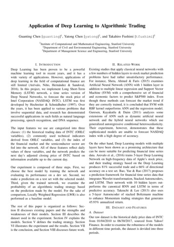
IV. M ETHODSA. Long Short-Term MemoryLong Short-Term Memory (LSTM) was first developedby Hochreiter & Schmidhuber (1997) as a variant ofRecurrent Neural Network (RNN). Over the years,LSTM has been applied to various problems thatinvolve sequential data, and research has demonstratedsuccessful applications in such fields as natural languageprocessing, speech recognition, and DNA sequence.Fig. 1: Stock price of Intel from 01/04/2010 to 06/30/2017. The blackarrows indicate the training sets, the red arrows indicate the dev sets,and the blue arrows indicate the of test sets.Period I ranges from 01/04/2010 to 06/29/2012. Period IIranges from 07/02/2012 to 12/31/2014. Period III rangesfrom 01/02/2015 to 06/30/2017. Furthermore, we divideeach sub-dataset into the training set, the dev set andthe test set, and the length of their periods is 2 years, 3months, and 3 months, respectively. The historical stockprice of INTC is shown in Figure 1, which also illustrateshow we split the data into the three different sets.B. Input FeaturesThe input features consist of three sets of variables. Thefirst set is the historical daily trading data of INTC including previous 5 day’s adjusted closing price, log returns,and OHLC variables. These features provide basic information about INTC stock. The second set is the technicalindicators that demonstrate various characteristics of thestock’s behavior. The third set is about indexes: S&P500,CBOE Volatility Index, and PHLX Semiconductor SectorIndex. Figure 2 describes the details of these variables.All of the inputs and output are scaled between 0 and 1before we feed them into the models.Like RNN, LSTM has a recurrent structure where eachcell not only outputs prediction ŷt but also transfersactivation ht to the next cell. The striking feature ofLSTM is its ability to store, forget, and read informationfrom the long-term state of the underlying dynamics,and these tasks are achieved through three types ofgates. In the forget gate, a cell receives long-term statect 1 , retains some pieces of the information by amountft , and then adds new memories that the input gateselected. The input gate determines what parts of thetransformed input gt need to be added to the long-termstate ct . This process updates long-term state ct , whichis directly transmitted to the next cell. Finally, outputgate transforms the updated long-term state ct throughtanh(·), filters it by ot , and produces the output ŷt ,which is also sent to the next cell as the short-term stateht .The equations for LSTM computations are given byTTit σ(Wxi· xt Whi· ht 1 bi )TTft σ(Wxf· xt Whf· ht 1 bf )TTot σ(Wxo· xt Who· ht 1 bo )TTgt tanh(Wxg· xt Whg· ht 1 bg )ct ft ct 1 it gtŷt ht ot tanh(ct )where is element-wise multiplication, σ(·) is thelogistic function, and tanh(·) is the hyperbolic tangentfunction. The three gates open and close according tothe value of the gate controllers ft , it , and ot , all ofwhich are fully connected layers of neurons. The rangeof their outputs is [0, 1] as they use the logistic functionfor activation. In each gate, their outputs are fed intoelement-wise multiplication operations, so if the outputis close to 0, the gate is narrowed and less memory isstored in ct , while if the output is close to 1, the gate ismore widely open, letting more memory flow throughthe gate. Given LSTM cells, it is common to stackmultiple layers of the cells to make the model deeperto be able to capture nonlinearity of the data. Figure 3illustrates how computation is carried out in a LSTM cell.Fig. 2: Descriptions of the input features [2]
The predicted value at the new target point x isŷ xT θ̂(x) xT (X T W (x)X) 1 X T W (x)y.Although the model is locally linear in y , computing ŷover the entire data set produces a curve that approximates the true function.V. T RADING S TRATEGYFig. 3: LSTM cell [3]We choose Mean Squared Error (MSE) with L2 regularization on the weights for the cost function:mL(θ) 1 X(yt ŷt )2mt 1 λ ( Wi 2 Wf 2 Wo 2 )where θ is the set of parameters to be trained includingthe weight matrices for each gate {Wi (Wxi ; Whi ),Wf (Wxf ; Whf ), Wo (Wxo ; Who )}, and the biasterms {bi , bf , bo , bg }.Since this is a RNN, LSTM is trained via Backpropagation Through Time. The key idea is that for eachcell, we first unroll the fixed number of previous cellsand then apply forward feed and backpropagation to theunrolled cells. The number of unrolled cells is anotherhyperparameter that needs to be selected in addition tothe number of neurons and layers.B. Locally Weighted Linear Regression:Locally Weighted Linear Regression is a nonparametricmodel that solves the following problem at each targetpoint x0 :1θ(x0 ) argmin (Xθ y)T W (x0 )(Xθ y).2θX Rm,n is the matrix of covariates, and y Rm is the outcome. The weight matrix W (x0 ) diag{w1 , · · · , wm } measures the closeness of x0 relativeto the observed points xt , t 1, · · · , m. The closer x0 isto xt , the higher the value of wt . The Gaussian kernel ischosen as the weight: (xt x0 )2wt (x0 ) exp 2τ 2where τ is a hyper parameter that controls the windowsize. The closed form solution of the optimization problem isθ̂(x0 ) (X T W (x0 )X) 1 X T W (x0 )y.We consider a simple algorithmic trading strategy basedon the prediction by the model. At day t, an investor buysone share of INTC stock if the predicted price is higherthan the current actual adjusted closing price. Otherwise,he or she sells one share of INTC stock. The strategy stcan be described as:( 1 if ŷt 1 ytst 1 if ŷt 1 ytwhere yt is the current adjusted closing price of INTCand ŷt 1 is the predicted price by the model. Using theindicator variable st , we can calculate a daily return ofthe strategy at day t 1: yt 1rt 1 st log cytwhere c denotes transaction cost, and the cumulativereturn from t 0 to m isr0m m 1Xrt .t 0We also consider the Sharpe Ratio to compare the profitability of the strategy with different models. The SharpeRatio is defined asSR E(r) rf.σ(r)E(r) is the expected return of a stock, rf is the risk-freerate, and σ(r) is the standard deviation of the return.VI. E XPERIMENT AND R ESULTSA. Setup for the ExperimentWe use TensorFlow to perform our experiment on thedataset. The choice of hyperparameters and optimizer arelisted in Table I:CategoriesLibraryOptimizerThe number of Hidden LayersThe number of Unrolled CellsThe number of NeuronsThe number of EpochsChoiceTensorFlowAdamOptimizer5102005000TABLE I: Hyperparameters/Optimizer for the LSTM Model
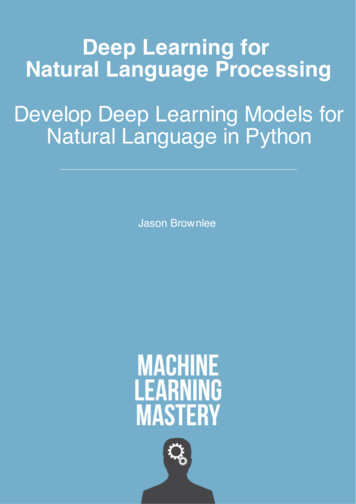
Fig. 4: MSE on the training and dev sets with different values of λ(The points indicate the lowest MSE on the dev set for each period)We choose 5 layers in line with the networks used byArevalo et al., (2016), Bao et al., (2017), and Takeuchi,& Lee (2013). Regarding the number of unrolled cells,10 (days) is assumed to be sufficient for the LSTMto predict the next day’s stock price and avoid thevanishing gradient problem. The number of neurons isdetermined by try and error.Since the architecture of the LSTM is 5 layers with200 neurons, which is deep and wide, it is necessaryto introduce regularization as discussed in SectionIV in order to avoid overfitting and improve thepredictive accuracy. For each period, we train thenetwork with different values of λ that controls thedegree of regularization and compute MSE on thetraining and dev set. The set of values of λ we consideris 0.1n (n 2, · · · , 8) and 0 that corresponds to noregularization. The MSE on the training and dev setswith different λ’s is illustrated in Figure 4. We select theλ that minimizes the MSE on dev set which is depictedas points in the plot.AdamOptimizer is selected because it is suitable fordeep learning problems with large dataset and manyparameters. As for the parameters of AdamOptimizer, weuse the default values provided by Tensorflow.B. The results of the experimentFig. 5: Predicted and actual price of Intel for three periods (scaled)the profitability of the algorithmic trading strategy.1) Mean Squared Error of Predicted Price:m1XMSE (yt ŷt )2mt 1where yt and ŷt denote the actual and predicted prices ofINTC at day t. The MSE of the both models are listed inTable II. The MSE of the LSTM on the test sets turns outto be small and lower than that of the LWR Models for allthe three periods. This result substantiates that the LSTMachieves higher predictive accuracy than the LWR.PeriodIIIIIITrain ErrorLSTMLWR0.00122 0.055710.00051 0.007020.00056 0.09385Dev ErrorLSTM LWR0.00436 0.106170.00984 0.044880.01568 0.03331Test ErrorLSTM LWR0.00564 0.053620.00772 0.015480.01146 0.02147Figure 5 shows the predicted stock price by both modelsand the actual price of INTC. The predicted prices ofthe LSTM are closer to the actual price than the ones ofthe LWR for all the three periods. It is important to notethat the LSTM seems to be able to predict the stockprice more accurately when the price does not exhibit aclear trend such as the first and third periods than whenthe price is boosting like the second period where theLSTM constantly underestimates it.1{·} is the indicator function. This measures the propor-To further evaluate the predictive performance of themodels, we calculate two measurements and examinetion of the days when the model forecasts the correctdirection of price movement. The DA on the test setis summarized in Table III. The LSTM accomplishesTABLE II: The MSE of the LSTM and LWR for the three periods2) Directional Accuracy:DA X1 m 11{(yt 1 yt )(ŷt 1 ŷt ) 0}m 1t 1
80.328% and 70.968% for the first and third periods,while the prediction by the LWR is slightly higher thanrandom guess in the same periods. The second period inwhich the price of INTC continued to rise appears to be achallenging moment for both models to make an 968LWR57.37745.90257.377TABLE III: Directional accuracy(%) of the LSTM and LWR for threeperiods3) Cumulative Daily Returns and Sharpe Ratio:r0m m 1Xrt and SR t 0E(r) rfσ(r)as defined in Section V. The cumulative daily returns andthe Sharpe Ratio for the strategy based on the LSTMand the LWR are shown in Table IV. The transactioncost of each trade is assumed to be 1 basis point. 13week treasury bill rate (IRX) is used as the risk-freerate. As a comparison, we also consider a Buy-and-Holdstrategy in which an investor buys one share of INTC atthe beginning of a test set and holds it until the end ofthe period. The LSTM-based strategy produces promisingcumulative returns and the Sharpe Ratio. In particular,the strategy yields a 54.8% cumulative daily return and a0.649 Sharpe Ratio during the first period despite the negative return of INTC (i.e., Buy-and-Hold strategy). TheLWR also generates higher returns and Sharpe Ratio thanthe Buy-and-Hold strategy, but the LSTM substantiallyoutperforms the LWR. Figure 6 illustrates the cumulativedaily returns of the strategies. The return of the LSTMbased strategy stably increases over time in the first andsecond periods.PeriodIIIIIILSTMReturns SR54.8%0.64928.6%0.25716.9%0.267LWRReturns SR25.5% 0.29215.3% 080.088-0.085TABLE IV: Cumulative daily returns and the Sharpe Ratio of thestrategies for three periodsVII. CONCLUSIONIn this project, we implement Long Short-Term MemoryNetwork to predict the stock price of INTC and applythe trained network to the algorithmic trading problem.The LSTM can accurately predict the next day’s price ofINTC especially when the stock price is lack of a trend.The strategy based on the prediction by the LSTM makespromising cumulative daily returns, outperforming theother two strategies. These results, however, are limitedFig. 6: Cumulative daily return of the Buy-and-Hold (blue line), theLSTM-based (green), and the LWR-based (red line) strategies.in some respects. We assume that it is always possibleto trade at the adjusted closing price every day, whichis not feasible in practice. Yet, our study demonstratesthe potential of LSTM in stock market prediction andalgorithmic trading.VIII. FUTURE WORKDue to the computational limitation, we were unableto conduct a comprehensive experiment to train variousarchitectures of the LSTM such as different numbers ofneurons and layers. Also, one of the biggest weaknessesof our LSTM is that it cannot capture a sheer trendlike the one observed in the test set of the secondperiod. Thus, a possible extension of our approach canbe to increase the number of layers to make the networkeven deeper and build the trading strategy combinedwith reinforcement learning that takes into account thecurrent state of the market. Another approach would beto make the network event-driven so that it can respondto structural changes in the financial market.IX. CONTRIBUTIONAll team members contributed to the progress of theproject. Specific work assignment is as follows. TakahiroFushimi implemented LSTM using TensorFlow, createdfigures, and wrote the final report. Yatong Chen wrote themilestone and final reports, performed analysis, and made
poster. Guanting Chen helped processing and testing data,advised machine learning methods, and implementedmachine learning models.R EFERENCES[1] Arévalo, A., Niño, J., Hernández, G., & Sandoval, J. (2016,August). High-frequency trading strategy based on deep neuralnetworks. In International conference on intelligent computing(pp. 424-436). Springer International Publishing.[2] Bao, W., Yue, J., & Rao, Y. (2017). A deep learning frameworkfor financial time series using stacked autoencoders and longshort term memory. PloS one, 12(7), e0180944.[3] Géron, A. (2017). Hands-on machine learning with ScikitLearn and TensorFlow: concepts, tools, and techniques to buildintelligent systems.[4] Guresen, E., Kayakutlu, G., & Daim, T. U. (2011). Usingartificial neural network models in stock market index prediction.Expert Systems with Applications, 38(8), 10389-10397.[5] Hochreiter, S., & Schmidhuber, J. (1997). Long short-termmemory. Neural computation, 9(8), 1735-1780.[6] Sheta, A. F., Ahmed, S. E. M., & Faris, H. (2015). A comparisonbetween regression, artificial neural networks and support vectormachines for predicting stock market index. Soft Computing, 7,8.[7] Takeuchi, L., & Lee, Y. Y. A. (2013). Applying deep learning toenhance momentum trading strategies in stocks. Working paper,Stanford University.
to enhance Momentum trading strategies that generates 45.93% annualized return. III. DATASET AND FEATURES A. Dataset Our raw dataset is the historical daily price data of INTC from 01/04/2010 to 06/30/2017, sourced from Yahoo! Finance. In order to examine the robustness of the models in diff