WIXLIB

1moment parameters θ {σ 2 , µcg , πa } to the parameters η(θ) {wcg σ2 µcg , bcg natural 2σ1 2 kµcg k22 , ba ln p(a) ln πa , b0 ln p(a 1)p(a 0) . The relationships η(θ) are referred to as thegenerative parameter constraints.We now demonstrate that the sequence of operations in the max-sum classifier in (3) coincides exactlywith the operations involved in one layer of a DCN: image normalization, linear template matching,thresholding, and max pooling. First, the image is normalized (by assumption). Second, the image isfiltered with a set of noise-scaled rendered templates wcg . If we assume translational invariance inthe RMM, then the rendered templates wcg yield a convolutional layer in a DCN [11] (see AppendixLemma A.2). Third, the resulting activations (log-probabilities of the hypotheses) are passed througha pooling layer; if g is a translational nuisance, then taking the maximum over g corresponds to maxpooling in a DCN. Fourth, since the switching variables are latent (unobserved), we max-marginalizeover them during classification. This leads to the ReLU operation (see Appendix Proposition A.3).3.2 The Deep Rendering Mixture Model: Capturing Levels of AbstractionMarginalizing over the nuisance g G in the RMM is intractable for modern datasets, since G willcontain all configurations of the high-dimensional nuisance variables g. In response, we extend theRMM into a hierarchical Deep Rendering Mixture Model (DRMM) by factorizing g into a number ofdifferent nuisance variables g (1) , g (2) , . . . , g (L) at different levels of abstraction. The DRMM imagegeneration process starts at the highest level of abstraction ( L), with the random choice of theobject class c(L) and overall nuisance g (L) . It is then followed by random choices of the lower-leveldetails g ( ) (we absorb the switching variable a into g for brevity), progressively rendering moreconcrete information level-by-level ( 1), until the process finally culminates in a fully renderedD-dimensional image I ( 0). Generation in the DRMM takes the form:c(L) Cat({πc(L) }), g ( ) Cat({πg( ) }) [L]µc(L) g (1)(2)(L 1) (L)Λg µc(L) Λg(1) Λg(2) · · · Λg(L 1) Λg(L) µc(L)N (µc(L) g , Ψ σ 2 1D ),(5)(6)I (7)where the latent variables, parameters, and helper variables are defined in full detail in Appendix B.The DRMM is a deep Gaussian Mixture Model (GMM) with special constraints on the latent variables.Here, c(L) C L and g ( ) G , where C L is the set of target-relevant nuisance variables, and G is theset of all target-irrelevant nuisance variables at level . The rendering path is defined as the sequence(c(L) , g (L) , . . . , g ( ) , . . . , g (1) ) from the root (overall class)Qdown to the individual pixels at 0.µc(L) g is the template used to render the image, and Λg Λg( ) represents the sequence of localnuisance transformations that partially render finer-scale details as we move from abstract to concrete.( )( )Note that each Λg( ) is an affine transformation with a bias term αg( ) that we have suppressed forclarity. Fig. 1B illustrates the corresponding graphical model. As before, we have suppressed thedependence of g ( ) on the pixel location x( ) at level of the hierarchy.Sum-Over-Paths Formulation of the DRMM. We can rewrite the DRMM generation processby expanding out the matrix multiplications into scalar products. This yields an interesting newP (L) (L)(1) (1)perspective on the DRMM, as each pixel intensity Ix p λp ap · · · λp ap is the sum over allactive paths to that pixel, of the product of weights along that path. A rendering path p is active iffQ ( )every switch on the path is active i.e. ap 1 . While exponentially many possible renderingpaths exist, only a very small fraction, controlled by the sparsity of a, are active. Fig. 1C depicts thesum-over-paths formulation graphically.Recursive and Nonnegative Forms. We can rewrite the DRMM into a recursive form as z ( ) ( 1)Λg( 1) z ( 1) , where z (L) µc(L) and z (0) I. We refer to the helper latent variables z ( ) asintermediate rendered templates. We also define the Nonnegative DRMM (NN-DRMM) as a DRMMwith an extra nonnegativity constraint on the intermediate rendered templates, z ( ) 0 [L].The latter is enforced in training via the use of a ReLu operation in the top-down reconstructionphase of inference. Throughout the rest of the paper, we will focus on the NN-DRMM, leaving theunconstrained DRMM for future work. For brevity, we will drop the NN prefix.Factor Model. We also define and explore a variant of the DRMM that where the top-level latentvariable is Gaussian: z (L 1) N (0, 1d ) Rd and the recursive generation process is otherwise4

( 1)identical to the DRMM: z ( ) Λg( 1) z ( 1) where g (L 1) c(L) . We call this the Deep RenderingFactor Model (DRFM). The DRFM is closely related to the Spike-and-Slab Sparse Coding model[25]. Below we explore some training results, but we leave most of the exploration for future work.(see Fig. 3 in Appendix C for architecture of the RFM, the shallow version of the DRFM)QNumber of Free Parameters.to the shallow RMM, which has D C L G parameters,P 1Comparedthe DRMM has only G D D 1 parameters, an exponential reduction in the number of freeparameters (Here G L 1 C L and D is the number of units in the -th layer with D0 D). Thisenables efficient inference, learning, and better generalization. Note that we have assumed dense(fully connected) Λg ’s here; if we impose more structure (e.g. translation invariance), the number ofparameters will be further reduced.Bottom-Up Inference. As in the shallow RMM, given an input image I the DRMM classifier infersthe most likely global configuration {c(L) , g ( ) }, 0, 1, . . . , L by executing the max-sum/productmessage passing algorithm in two stages: (i) bottom-up (from fine-to-coarse) to infer the overall classlabel ĉ(L) and (ii) top-down (from coarse-to-fine) to infer the latent variables ĝ ( ) at all intermediatelevels . First, we will focus on the fine-to-coarse pass since it leads directly to DCNs.Using (3), the fine-to-coarse NN-DRMM inference algorithm for inferring the most likely cateogryĉL is given byargmax max µTc(L) g I argmax max µTc(L)c(L) Cg Gc(L) C argmaxc(L) CµTc(L)g Gmaxg (L) G LΛTg(L)1YΛTg( ) I L· · · max ΛTg(1) I · · · argmax µTc(L) I (L) . (8)g (1) G 1c(L) C{z} I1Here, we have assumed the bias terms αg( ) 0. In the second line, we used the max-productalgorithm (distributivity of max over products i.e. for a 0, max{ab, ac} a max{b, c}). SeeAppendix B for full details. This enables us to rewrite (8) recursively:I ( 1) maxg ( 1) G 1(Λg( 1) )T I ( ) MaxPool(ReLu(Conv(I ( ) ))), {z }(9) W ( 1)where I ( ) is the output feature maps of layer , I (0) I and W ( ) are the filters/weights for layer .Comparing to (3), we see that the -th iteration of (8) and (9) corresponds to feedforward propagationin the -th layer of a DCN. Thus a DCN’s operation has a probabilistic interpretation as fine-to-coarseinference of the most probable configuration in the DRMM.Top-Down Inference. A unique contribution of our generative model-based approach is that we havea principled derivation of a top-down inference algorithm for the NN-DRMM (Appendix B). Theresulting algorithm amounts to a simple top-down reconstruction term Iˆn Λĝn µĉ(L) .nDiscriminative Relaxations: From Generative to Discriminative Classifiers. We have constructed a correspondence between the DRMM and DCNs, but the mapping is not yet complete.In particular, recall the generative constraints on the weights and biases. DCNs do not have suchconstraints — their weights and biases are free parameters. As a result, when faced with training datathat violates the DRMM’s underlying assumptions, the DCN will have more freedom to compensate.In order to complete our mapping from the DRMM to DCNs, we relax these parameter constraints,allowing the weights and biases to be free and independent parameters. We refer to this process as adiscriminative relaxation of a generative classifier ([16, 4], see the Appendix D for details).3.3 Learning the Deep Rendering Model via the Expectation-Maximization (EM) AlgorithmWe describe how to learn the DRMM parameters from training data via the hard EM algorithm inAlgorithm 1.The DRMM E-Step consists of bottom-up and top-down (reconstruction) E-steps at each layer inthe model. The γncg p(c, g In ; θ) are the responsibilities, where for brevity we have absorbed ainto g. The DRMM M-step consists of M-steps for each layer in the model. The per-layer M-stepin turn consists of a responsibility-weighted regression, where GLS(yn xn ) denotes the solutionto a generalized Least Squares regression problem that predict targets yn from predictors xn and is5

Algorithm 1 Hard EM and EG Algorithms for the DRMME-step:M-step:G-step:ĉn , ĝn argmax γncgc,g Λ̂g( ) {z}GLS In( 1) ẑn( ) g ( ) ĝn( ) g ( ) Λ̂g( ) Λg( ) DRM M (θ)closely related to the SVD. The Iversen bracket is defined as JbK 1 if expression b is true and is 0otherwise.There are several interesting and useful features of the EM algorithm. First, we note that it is aderivative-free alternative to the back propagation algorithm for training that is both intuitive andpotentially much faster (provided a good implementation for the GLS problem). Second, it is easilyparallelized over layers, since the M-step updates each layer separately (model parallelism). Moreover,it can be extended to a batch version so that at each iteration the model is simultaneously updatedusing separate subsets of the data (data parallelism). This will enable training to be distributed easilyacross multiple machines. In this vein, our EM algorithm shares several features with the ADMMbased Bregman iteration algorithm in [31]. However, the motivation there is from an optimizationperspective and so the resulting training algorithm is not derived from a proper probabilistic density.Third, it is far more interpretable via its connections to (deep) sparse coding and to the hard EMalgorithm for GMMs. The sum-over-paths formulation makes it particularly clear that the mixturecomponents are paths (from root to pixels) in the DRMM.G-step. For the training results in this paper, we use the Generalized EM algorithm wherein wereplace the M-step with a gradient descent based G-step (see Algorithm 1). This is useful forcomparison with backpropagation-based training and for ease of implementation. But before we usethe G-step, we would like to make a few remarks about the proper M-step of the algorithm, savingthe implementation for future work.Flexibility and Extensibility. Since we can choose different priors/types for the nuisances g, thelarger DRMM family could be useful for modeling a wider range of inputs, including scenes, speechand text. The EM algorithm can then be used to train the whole system end-to-end on differentsources/modalities of labeled and unlabeled data. Moreover, the capability to sample from the modelallows us to probe what is captured by the DRMM, providing us with principled ways to improve themodel. And finally, in order to properly account for noise/uncertainty, it is possible in principle toextend this algorithm into a soft EM algorithm. We leave these interesting extensions for future work.3.4New Insights into Deep ConvnetsDCNs are Message Passing Networks. The DRMM inference algorithm is equivalent to performingmax-sum-product message passing of the DRMM Note that by “max-sum-product” we mean a novelcombination of max-sum and max-product as described in more detail in the proofs in the Appendix.The factor graph encodes the same information as the generative model but organizes it in a mannerthat simplifies the definition and execution of inference algorithms [10]. Such inference algorithmsare called message passing algorithms, because they work by passing real-valued functions calledmessages along the edges between nodes. In the DRMM, the messages sent from finer to coarser levelsare in fact the feature maps I ( ) . The factor graph formulation provides a powerful interpretation: theconvolution, Max-Pooling and ReLu operations in a DCN correspond to max-sum/product inferencein a DRMM. Thus, we see that architectures and layer types commonly used in today’s DCNs can bederived from precise probabilistic assumptions that entirely determine their structure. The DRMMtherefore unifies two perspectives — neural network and probabilistic inference (see Table 2 in theAppendix for details).Shortcomings of DCNs. DCNs perform poorly in categorizing transparent objects [23]. Thismight be explained by the fact that transparent objects generate pixels that have multiple sources,conflicting with the DRMM sparsity prior on a, which encourages few sources. DCNs also fail toclassify slender and man-made objects [23]. This is because of the locality imposed by the locally6

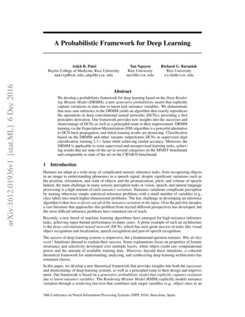
connected/convolutional layers, or equivalently, the small size of the template µc(L) g in the DRMM.As a result, DCNs fail to model long-range correlations.Class Appearance Models and Activity Maximization. The DRMM enables us to understand howtrained DCNs distill and store knowledge from past experiences in their parameters. Specifically, theDRMM generates rendered templates µc(L) g via a mixture of products of affine transformations, thusimplying that class appearance models in DCNs are stored in a similar factorized-mixture form overmultiple levels of abstraction. As a result, it is the product of all the filters/weights over all layersthat yield meaningful images of objects (Eq. 7). We can also shed new light on another approachto understanding DCN memories that proceeds by searching for input images that maximize theactivity of a particular class unit (say, class of cats) [26], a technique we call activity maximization.Results from activity maximization on a high performance DCN trained on 15 million images isshown in Fig. 1 of [26]. The resulting images reveal much about how DCNs store memories. Usingthe DRMM, the solution Ic (L) of the activity maximization for class c(L) can be derived as the sumof individual activity-maximizing patches IP i , each of which is a function of the learned DRMMparameters (see Appendix E):XX Ic (L) IP i (c(L) , gP) µ(c(L) , gP).(10)iiPi PPi PThis implies thatcontains multiple appearances of the same object but in various poses. Each activity-maximizing patch has its own pose gP, consistent with Fig. 1 of [26] and our own extensiveiexperiments with AlexNet, VGGNet, and GoogLeNet (data not shown). Such images provide strongconfirmational evidence that the underlying model is a mixture over nuisance parameters, as predctedby the DRMM.Ic (L)Unsupervised Learning of Latent Task Nuisances. A key goal of representation learning is todisentangle the factors of variation that contribute to an image’s appearance. Given our formulation ofthe DRMM, it is clear that DCNs are discriminative classifiers that capture these factors of variationwith latent nuisance variables g. As such, the theory presented here makes a clear prediction that fora DCN, supervised learning of task targets will lead to unsupervised learning of latent task nuisancevariables. From the perspective of manifold learning, this means that the architecture of DCNs isdesigned to learn and disentangle the intrinsic dimensions of the data manifolds.In order to test this prediction, we trained a DCN to classify synthetically rendered images ofnaturalistic objects, such as cars and cats, with variation in factors such as location, pose, and lighting.After training, we probed the layers of the trained DCN to quantify how much linearly decodableinformation exists about the task target c(L) and latent nuisance variables g. Fig. 2 (Left) shows thatthe trained DCN possesses significant information about latent factors of variation and, furthermore,the more nuisance variables, the more layers are required to disentangle the factors. This is strongevidence that depth is necessary and that the amount of depth required increases with the complexityof the class models and the nuisance variations.4Experimental ResultsWe evaluate the DRMM and DRFM’s performance on the MNIST dataset, a standard digit classification benchmark with a training set of 60,000 28 28 labeled images and a test set of 10,000 labeledimages. We also evaluate the DRMM’s performance on CIFAR10, a dataset of natural objects whichinclude a training set of 50,000 32 32 labeled images and a test set of 10,000 labeled images. In allexperiments, we use a full E-step that has a bottom-up phase and a principled top-down reconstructionphase. In order to approximate the class posterior in the DRMM, we include a Kullback-Leiblerdivergence term between the inferred posterior p(c I) and the true prior p(c) as a regularizer [9].We also replace the M-step in the EM algorithm of Algorithm 1 by a G-step where we updatethe model parameters via gradient descent. This variant of EM is known as the Generalized EMalgorithm [3], and here we refer to it as EG. All DRMM experiments were done with the NN-DRMM.Configurations of our models and the corresponding DCNs are provided in the Appendix I.Supervised Training. Supervised training results are shown in Table 3 in the Appendix. ShallowRFM: The 1-layer RFM (RFM sup) yields similar performance to a Convnet of the same configuration(1.21% vs. 1.30% test error). Also, as predicted by the theory of generative vs discriminativeclassifiers, EG training converges 2-3x faster than a DCN (18 vs. 40 epochs to reach 1.5% test error,Fig. 2, middle). Deep RFM: Training results from an initial implementation of the 2-layer DRFM7

Pretraining Finetune End-to-EndSupervisedSemisupervised1-layer ConvnetTest er Convnet0.08Test 00.000102030Epoch4050Figure 2: Information about latent nuisance variables at each layer (Left), training results from EGfor RFM (Middle) and DRFM (Right) on MNIST, as compared to DCNs of the same configuration.EG algorithm converges 2 3 faster than a DCN of the same configuration, while achieving asimilar asymptotic test error (Fig. 2, Right). Also, for completeness, we compare supervised trainingfor a 5-layer DRMM with a corresponding DCN, and they show comparable accuracy (0.89% vs0.81%, Table 3).Unsupervised Training. We train the RFM and the 5-layer DRMM unsupervised with NU images,followed by an end-to-end re-training of the whole model (unsup-pretr) using NL labeled images. Theres

theoretical framework for understanding, analyzing, and synthesizing deep learning architectures has remained elusive. In this paper, we develop a new theoretical framework that provides insights into both the successes and shortcomings of deep learning systems, as wel