Transcription
Copyright 2010 IEEE. Reprinted from “2010 Reliability andMaintainability Symposium,” San Jose, CA, USA, January 2528, 2010.This material is posted here with permission of the IEEE. Suchpermission of the IEEE does not in any way imply IEEEendorsement of any of ReliaSoft Corporation's products orservices. Internal or personal use of this material is permitted.However, permission to reprint/republish this material foradvertising or promotional purposes or for creating newcollective works for resale or redistribution must be obtainedfrom the IEEE by writing to pubs-permissions@ieee.org.By choosing to view this document, you agree to all provisionsof the copyright laws protecting it.
2010 Annual RELIABILITY and MAINTAINABILITY SymposiumDesign of Experiments and Data AnalysisHuairui Guo, Ph. D. & Adamantios MettasHuairui Guo, Ph.D., CPR.ReliaSoft Corporation1450 S. Eastside LoopTucson, AZ 85710 USAe-mail: Harry.Guo@ReliaSoft.comAdamantios Mettas, CPRReliaSoft Corporation1450 S. Eastside LoopTucson, AZ 85710 USAe-mail: Adam.Mettas@ReliaSoft.comTutorial Notes 2010 AR&MS
SUMMARY & PURPOSEDesign of Experiments (DOE) is one of the most useful statistical tools in product design and testing. While manyorganizations benefit from designed experiments, others are getting data with little useful information and wasting resourcesbecause of experiments that have not been carefully designed. Design of Experiments can be applied in many areas includingbut not limited to: design comparisons, variable identification, design optimization, process control and product performanceprediction. Different design types in DOE have been developed for different purposes. Many engineers are confused or evenintimidated by so many options.This tutorial will focus on how to plan experiments effectively and how to analyze data correctly. Practical and correctmethods for analyzing data from life testing will also be provided.Huairui Guo, Ph.D., CRPHuairui Guo is the Director of Theoretical Development at ReliaSoft Corporation. He received his Ph.D. in Systems andIndustrial Engineering from the University of Arizona. He has published numerous papers in the areas of quality engineeringincluding SPC, ANOVA and DOE and reliability engineering. His current research interests include repairable systemmodeling, accelerated life/degradation Testing, warranty data analysis and robust optimization. Dr. Guo is a member of SRE,IIE and IEEE. He is a Certified Reliability Professional (CRP).Adamantios Mettas, CRPMr. Mettas is the Vice President of product development at ReliaSoft Corporation. He fills a critical role in the advancement ofReliaSoft's theoretical research efforts and formulations in the subjects of Life Data Analysis, Accelerated Life Testing, andSystem Reliability and Maintainability. He has played a key role in the development of ReliaSoft's software including,Weibull , ALTA and BlockSim, and has published numerous papers on various reliability methods. Mr. Mettas holds a B.Sdegree in Mechanical Engineering and an M.S. degree in Reliability Engineering from the University of Arizona. He is aCertified Reliability Professional (CRP).Table of Contents1.2.3.4.5.6.7.8.Introduction .1Statistical Background .2Two Level Factorial Design .3Response Surface Methods (RSM) .6DOE for Life Testing .9Conclusions .10References .11Tutorial Visuals . .12ii – Guo & Mettas2010 AR&MS Tutorial Notes
1.INTRODUCTIONThe most effective way to improve product quality andreliability is to integrate them in the design and manufacturingprocess. Design of Experiments (DOE) is a useful tool that canbe integrated into the early stages of the development cycle. Ithas been successfully adopted by many industries, includingautomotive, semiconductor, medical devices, chemicalproducts, etc. The application of DOE is not limited toengineering. Many successful stories can be found in otherareas. For example, it has been used to reduce administrationcosts, improve the efficiency of surgery processes, andestablish better advertisement strategies.1.1 Why DOEDOE will make your life easier. For many engineers,applying DOE knowledge in their daily work will reduce lotsof trouble. Here are two examples of bad experiments that willcause trouble.Example 1: Assume the reliability of a product is affected byvoltage. The usage level voltage is 10. In order to predict thereliability at the usage level, fifty units are available foraccelerated life testing. An engineer tested all fifty units at avoltage of 25. Is this a good test?Example 2: Assume the reliability of a product is affected bytemperature and humidity. The usage level is 40 degreesCelsius and 50% relative humidity. In order to predict thereliability at the usage level, fifty units are available foraccelerated life testing. The design is conducted in thefollowing way:Number 5Table 1 – Two Stress Accelerated Life TestWill the engineer be able to predict the reliability at the usagelevel with the failure data from this test?1.2 What DOE Can DoDOE can help you design better tests than the above twoexamples. Based on the objectives of the experiments, DOEcan be used for the following purposes [1, 2]:1. Comparisons. When you have multiple design options,several materials or suppliers are available, you can design anexperiment to choose the best one. For example, in thecomparison of six different suppliers that provide connectors,will the components have the same expected life? If they aredifferent, how are they different and which is the best?2. Variable Screening. If there are a large number ofvariables that can affect the performance of a product or asystem, but only a relatively small number of them areimportant, a screening experiment can be conducted toidentify the important variables. For example, the warrantyreturn is abnormally high after a new product is launched.Variables that may affect the life are temperature, voltage,duty cycle, humidity and several other factors. DOE can beused to quickly identify the troublemakers and a follow-upexperiment can provide the guidelines for design modificationto improve the reliability.3. Transfer Function Exploration. Once a small number ofvariables have been identified as important, their effects on thesystem performance or response can be further explored. Therelationship between the input variables and output response iscalled the transfer function. DOE can be applied to designefficient experiments to study the linear and quadratic effectsof the variables and some of the interactions between thevariables.4. System Optimization. The goal of system design is toimprove the system performance, such as to improve theefficiency, quality, and reliability. If the transfer functionbetween variables and responses has been identified, thetransfer function can be used for design optimization. DOEprovides an intelligent sequential strategy to quickly move theexperiment to a region containing the optimum settings of thevariables.5. System Robustness. In addition to optimizing theresponse, it is important to make the system robust against“noise,” such as environmental factors and uncontrolledfactors. Robust design, one of the DOE techniques, can beused to achieve this goal.1.3 Common Design TypesDifferent designs have been used for different experimentpurposes. The following list gives the commonly used designtypes.1. For comparison One factor design2. For variable screening 2 level factorial design Taguchi orthogonal array Plackett-Burman design3. For transfer function identification and optimization Central composite design Box-Behnken design4. For system robustness Taguchi robust designThe designs used for transfer function identification andoptimization are called Response Surface Method designs. Inthis tutorial, we will focus on 2 level factorial design andresponse surface method designs. They are the two mostpopular and basic designs.1.4 General Guidelines for Conducting DOEDOE is not only a collection of statistical techniques thatenable an engineer to conduct better experiments and analyzedata efficiently; it is also a philosophy. In this section, generalguidelines for planning efficient experiments will be given.The following seven-step procedure should be followed [1, 2].1. Clarify and State Objective. The objective of theexperiment should be clearly stated. It is helpful to prepare a2010 Annual RELIABILITY and MAINTAINABILITY SymposiumGuo & Mettas – 1
list of specific problems that are to be addressed by theexperiment.2. Choose Responses. Responses are the experimentaloutcomes. An experiment may have multiple responses basedon the stated objectives. The responses that have been chosenshould be measurable.3. Choose Factors and Levels. A factor is a variable that isgoing to be studied through the experiment in order tounderstand its effect on the responses. Once a factor has beenselected, the value range of the factor that will be used in theexperiment should be determined. Two or more values withinthe range need to be used. These values are referred to aslevels or settings. Practical constraints of treatments must beconsidered, especially when safety is involved. A cause-andeffect diagram or a fishbone diagram can be utilized to helpidentify factors and determine factor levels.4. Choose Experimental design. According to the objectiveof the experiments, the analysts will need to select the numberof factors, the number of level of factors, and an appropriatedesign type. For example, if the objective is to identifyimportant factors from many potential factors, a screeningdesign should be used. If the objective is to optimize theresponse, designs used to establish the factor-responsefunction should be planned. In selecting design types, theavailable number of test samples should also be considered.5. Perform the Experiment. A design matrix should be usedas a guide for the experiment. This matrix describes theexperiment in terms of the actual values of factors and the testsequence of factor combinations. For a hard-to-set factor, itsvalue should be set first. Within each of this factor’s settings,the combinations of other factors should be tested.6. Analyze the Data. Statistical methods such as regressionanalysis and ANOVA (Analysis of Variance) are the tools fordata analysis. Engineering knowledge should be integratedinto the analysis process. Statistical methods cannot prove thata factor has a particular effect. They only provide guidelinesfor making decisions. Statistical techniques together with goodengineering knowledge and common sense will usually lead tosound conclusions. Without common sense, pure statisticalmodels may be misleading. For example, models created bysmart Wall Street scientists did not avoid, and probablycontributed to, the economic crisis in 2008.7. Draw Conclusions and Make Recommendations. Once thedata have been analyzed, practical conclusions andrecommendations should be made. Graphical methods areoften useful, particularly in presenting the results to others.Confirmation testing must be performed to validate theconclusion and recommendations.The above seven steps are the general guidelines forperforming an experiment. A successful experiment requiresknowledge of the factors, the ranges of these factors and theappropriate number of levels to use. Generally, thisinformation is not perfectly known before the experiment.Therefore, it is suggested to perform experiments iterativelyand sequentially. It is usually a major mistake to design asingle, large, comprehensive experiment at the start of a study.2 – Guo & MettasAs a general rule, no more than 25 percent of the availableresources should be invested in the first experiment.2.STATISTICAL BACKGROUNDLinear regression and ANOVA are the statistical methodsused in DOE data analysis. Knowing them will help you havea better understand of DOE.2.1 Linear Regression[2]A general linear model or a multiple regression model is:(1)Y β 0 β1 X 1 . β p X p εWhere: Y is the response also called output or dependentvariable. X i is the predictor also called input or independentvariable. ε is the random error or noise, which is assumed tobe normally distributed with mean 0 and variance σ 2 , usuallynoted as ε N (0, σ 2 ) . Because ε is normally distributed,then for a given value of X, Y is also normally distributed andVar (Y ) σ 2 .From the model, it can be seen that the variation or thedifference of Y consists of two parts. One is the random part ofε . The other is the difference caused by the difference of theX values. For example, consider the data in Table 90512095400612095430YMean325170415Table 2 – Example Data for Linear RegressionTable 2 has three different combinations of X1 and X2,showing at different colors. For each combination, there aretwo observations. Because of the randomness caused by ε ,these two observations are different although they have thesame X values. This difference usually is called within-runvariation. The mean values of Y at the three combinations aredifferent too. This difference is caused by the difference of X1and X2 and usually is called between-run variation.If the between-run variation is significantly larger than thewithin-run variation, it means most of the variation of Y iscaused by the difference of X settings. In other words, Xssignificantly affect Y. The difference of Ys caused by the Xsare much more significant than the difference caused by thenoise.From Table 2, we have the feeling that the between-runvariation is larger than the within-run variation. To confirmthis, statistical methods should be applied. The amount of thetotal variation of Y is defined by the sum of squares:n(SST Yi Yi 1)2(2)Where Yi is the ith observed value and Y is the mean of all2010 AR&MS Tutorial Notes
the observations. However, since SST is affected by thenumber of observations, to eliminate this effect, anothermetric called mean squares is used to measure the normalizedvariability of Y.SS1 n2(3)MST T Yi Yn 1 n 1 i 1()Equation (3) is also the unbiased estimator of Var (Y ) .As mentioned before, the total sum of squares can bepartitioned into two parts: within-run variation caused byrandom noise (called sum of squares of error SS E ) and thebetween-run variation caused by different values of Xs (calledsum of squares of regression SS R ).nni 1i 1SS T SS R SS E (Yˆi Y ) 2 (Yi Yˆi ) 2(4)Where: Yˆi is the predicted value for the ith test. For tests withthe same X values, the predicted values are the same.Similar to equation (3), the mean squares of regressionand the mean squares of error are calculated by:2SS1 n(5)MS R R Yˆi Ypp i 1(MS E )(nSS E1 Yi Yˆi n 1 p n 1 p i 1)2(6)Where: p is the number of Xs.When there is more than one input variable, SS R can befurther divided into the variation caused by each variable, suchas:(7)SS R SS X1 SS X 2 . SS X pThe mean squares of each input variable MS X i is comparedwith MS E to test if the effect of X i is significantly greaterthan the effect of noise.The mean squares of regression MS R is used to measurethe between-run variance that is caused by predictor Xs. Themean squares of error MS E represents the within-run variancecaused by noise. By comparing these two values, we can findout if the variance contributed by Xs is significantly greaterthan the variance caused by noise. ANOVA is the methodused for the comparison in a statistical way.2.2 ANOVA (Analysis of Variance)can easily verify that:SST SS R SS E SS X1 SS X 2 SS EThe fifth column shows the F ratio of each source. All thevalues are much bigger than 1. The last column is the P value.The smaller the P value is, the larger the difference betweenthe variance caused by the corresponding source and thevariance caused by noise. Usually, a significance level α ,such as 0.05 or 0.1 is used to compare with the P values. If aP value is less than α , the corresponding source is said to besignificant at the significance level of α . From Table 3, wecan see that both variables X1 and X2 are significant to theresponse Y at the significance level of 0.1.MS R(8)MS Eis used to test the following two hypotheses:H0: There is no difference between the variance causedby Xs and the variance caused by noise.H1: The variance caused by Xs is larger than the variancecaused by noise.Under the null hypothesis, the ratio follows the F distributionwith degree of freedoms of p and n 1 p . By applyingANOVA to the data for this example, we get the followingANOVA table.The third column shows the values for the sum of squares. WeDegreesofFreedomSource ofVariationSum ofSquaresMeanSquaresFRatioPValueModel26.14E 043.07E 0436.860.0077X116.00E 046.00E .3333Total56.39E 04Table 3 – ANOVA Table for the Linear Regression ExampleAnother way to test whether or not a variable issignificant is to test whether or not its coefficient is 0 in theregression model. For this example, the linear regressionmodel is:(10)Y β 0 β1 X 1 β1 X 2 εIf we want to test whether or not β1 0 , we can use thefollowing hypothesis:H0: β1 0Under this null hypothesis, the statistic is a t distribution:β1(11)se( β1 )Se( β1 ) is the standard error of β1 that is estimated from thedata. The t test results are given in Table 4.T0 TermCoefficientStandard ErrorT ValueP .4870.0034X2185.77353.11770.0526The following ratioF0 (9)Table 4 – Coefficients for the Linear Regression ExampleTable 3 and Table 4 give the same P values.With linear regression and ANOVA in mind, we can startdiscussing DOE now.3.TWO LEVEL FACTORIAL DESIGNSTwo level factorial designs are used for factor screening.In order to study the effect of a factor, at least two differentsettings for this factor are required. This also can be explainedfrom the viewpoint of linear regression. To fit a line, twopoints are the minimal requirement. Therefore, the engineer2010 Annual RELIABILITY and MAINTAINABILITY SymposiumGuo & Mettas – 3
who tested all the units at a voltage of 25 will not be able topredict the life at the usage level of 10 volts. With only onevoltage value, the effect of voltage cannot be evaluated.3.1 Two Level Full Factorial DesignWhen the number of factors is small and you have theresources, a full factorial design should be conducted. Herewe will use a simple example to introduce some basicconcepts in DOE.For an experiment with two factors, the factors usually arecalled A and B. Uppercase letters are used for factors. Thefirst level or the low level is represented by -1, while thesecond level or the high level is represented by 1. There arefour combinations of a 2 level 2 factorial design. Eachcombination is called a treatment. Treatments are representedby lowercase letters. The number of test units for eachtreatment is called the number of replicates. For example, ifyou test two samples at each treatment, the number ofreplicates is 2. Since the number of replicates for each factorcombination is the same, this design is also balanced. A twolevel factorial design with k factors usually is written as 2 kdesign and read as “2 to the power of 3 design” or “2 to the 3design.” For a 2 2 design, the design matrix 13520Table 5 – Treatments for 2 Level Factorial DesignThis design is orthogonal. This is because the sum of theproductofAandBiszero,whichisAnorthogonal( 1 1) (1 1) ( 1 1) (1 1) 0 .design will reduce the estimation uncertainty of the modelcoefficients.The following linear regression model is used for theanalysis:(12)Y β 0 β1 X 1 β 2 X 2 β12 X 1 X 2 εWhere: X 1 is for factor A; X 2 is for factor B; and theirinteraction is represented by X 1 X 2 . The effects of A and Bare called main effects. The effects of their interaction arecalled two-way interaction effects. These three effects are thethree sources for the variation of Y. Since equation (12) is alinear regression model, the ANOVA method and the t-testgiven in Section 2 can be used to test whether or not one effectis significant.For a balanced design, a simple way to calculate the effectof a factor is to calculate the difference of the mean values ofthe response at its high and low setting. For example, theeffect of A can be calculated by:4 – Guo & MettasEffet of A Avg. at A high - Avg. at A low (13)30 35 20 25 10223.2 Two Level Fractional Factorial DesignWhen you increase the number of factors, the number oftest units will increase quickly. For example, to study 7factors, 128 units are needed. In reality, responses are affectedby a small number of main effects and lower orderinteractions. Higher order interactions are relativelyunimportant. This statement is called the sparsity of effectsprinciple. According to this principle, fractional factorialdesigns are developed. These designs use fewer samples toestimate main effects and lower order interactions, while thehigher order interactions are considered to have negligibleeffects.Consider a 2 3 design. 8 test units are required for a fullfactorial design. Assume only 4 test units are availablebecause of the cost of the test. Which 4 of the 8 treatmentsshould you choose? A full design matrix with all the effectsfor a 2 3 design 11-181111111Table 6 – Design Matrix for a 2 3 DesignIf the effect of ABC can be ignored, the following 4treatments can be used in the 115-1-111-1-1181111111Table 7 –Fraction of the Design Matrix for a 2 3 DesignIn Table 7, the effect of ABC cannot be estimated from theexperiment because it is always at the same level of 1. SinceTable 7 uses only half of the treatments from the full factorialdesign in Table 6, it is represented by 2 3 1 and read as “2 tothe power of 3 minus 1 design” or “2 to the 3 minus 1 design.”From Table 7, you will also notice that some columnshave the same values. For example, column AB and C are thesame. Using equation (13) to calculate the effect of AB and C,we will end up with the same procedure and result. Therefore,from this experiment, the effect of AB and C cannot be2010 AR&MS Tutorial Notes
distinguished because they change with the same pattern. InDOE, effects that cannot be separated from an experiment arecalled confounded effects or aliased effects. A list of aliasedeffects is called the alias structure. For the design of Table 7,the alias structure is:[I] I ABC; [A] A AC; [B] B BC; [C] C ABWhere: I is the effect of the intercept in the regression model,which represents the mean value of the response. The alias forI is called the defining relation. For this example, the definingrelation is written as I ABC. In a design, I may be aliasedwith several effects. The order of the shortest effects thataliased with I is the “resolution” of this design.From the alias structure, we can see that main effects areconfounded with 2-way interactions. For example, theestimated effect for C in fact is the combination effect of Cand AB.Checking Table 7, we can see it is a full factorial design ifwe have only factor A and B. Therefore, A and B usually arecalled basic factors and the full factorial design for them iscalled the basic design. A fractional factorial design isgenerated from its basic design and basic factor. For thisexample, the values for factor C are generated from the valuesof the basic factors A and B using the relation C AB. UsuallyAB is called the factor generator for C.By now, it should be clear that the design given in Table 1at the beginning of this tutorial is not a good design. If youcheck the design in terms of coded value, the answer isobvious. Table 8 shows the design again.Number ofUnitsTemperature(Celsius)25120 (1)95 (1)2585 (-1)85 (-1)AAperture SettingsmalllargeBExposure Timeminutes2040CDevelop Timeseconds3045DMask DimensionsmalllargeEEtch Time14.515.5Table 9 –Factor Settings for a Five Factor ExperimentWith five factors the total number of runs required for afull factorial is 2 5 32 . Running all of the 32 combinations istoo expensive for the manufacturer. At the initialinvestigation, only main effects and two factor interactions areof interest, while higher order interactions are considered to beunimportant. It is decided to carry out the investigation usingthe 2 5 1 design, which requires 16 runs. The defining relationis I ABCDE, or in other words, the generator for factor E isE ABCD. Table 10 gives the experiment data.Run 5.563Humidity(%)Table 8 – Two Stress Accelerated Life Test (Coded Value)In this design, temperature and humidity are confounded. Infact, to study the effect of two factors, at least three differentsettings are required. From the linear regression point of view,at least three unique settings are needed to solve threeparameters: the intercept, the effect of factor A and the effectof factor B. If their interaction is also to be estimated, fourdifferent settings should be used. Many DOE softwarepackages can generate a design matrix for you according tothe number of factors and the level of factors. It will help youavoid bad designs such as the one given in Table 8.Table 10 –Design Matrix and ResultsSince the design has only 16 unique factor combinations, itcan be used to estimate only 16 parameters in the linearregression model. If we include all main and 2-wayinteractions in the model, we get the following ANOVA table.3.3 An Example of a Fractional Factorial DesignAssume an engineer wants to identify the factors thataffect the yield of a manufacturing process for integratedcircuits. By following the DOE guidelines, five factors arebrought up and a two level fractional factorial design isdecided to be used [1]. The five factors and their levels aregiven in Table 9.FactorNameUnitLow(-1)minutesHigh(1)2010 Annual RELIABILITY and MAINTAINABILITY SymposiumSource ofVariationDFSum --Guo & Mettas – 5
2.5625Lack of Fit39.68753.2292Pure Error818.52.3125155775.4375ABTotal5775.4375Table 11 –ANOVA Table with All EffectsTable 12 –ANOVA Table with Significant EffectsThere are no F ratio and P values in the above table. This isbecause there are no replicates in this experiment when all theeffects are considered. Therefore, there is no way to estimatethe error term in the regression model. This is why the SSE(Sum of Squares of Error), labeled as Residual in Table 11, is0. Without SSE, the estimation of the random error, how canwe test whether or not an effect is significant compared torandom error? Don’t panic. Statisticians have alreadydeveloped methods to deal with this situation. When there isno error in a screening experiment, Lenth’s method can beused to identify significant effects. Lenth’s method assumesthat all the effects should be normally distributed with a meanof 0, given the hypothesis that they are not significant. If anyeffects are significantly different from 0, they should beconsidered significant. So we can check the normal probabilityplot for effects.From Table 12, we can see that effects A, B, C and AB areindeed significant because their P values are close to 0.Once the important factors have been identified, followup experiments can be conducted to optimize the process.Response Surface Methods are developed for this purpose.ReliaSoft DOE - www.ReliaSoft.comNormal ProbabilityPlot of Effect99.000Effect ProbabilityB:Exposure TimeA:Aperture SettingYieldY' YNon-Significant EffectsSignificant EffectsDistribution LineC:Develop 000-8.0008.00024.000QAReliasoft7/10/20093:03:18 PM40.000EffectAlpha 0.1; Lenth's PSE 0.9375Figure 1-Effect Probability Plot Using Lenth’s MethodFrom Figure 1, the main effect A, B, C and the 2-wayinteraction AB are identified as sig
Design of Experiments (DOE) is one of the most useful statistical tools in product design and testing. While many organizations benefit from designed experiments, others are getting data with little useful information and wasting resources because of ex