Transcription
Digital Image u/farid
0. History of Photo Tampering0.1: History . . . . . . . . . . . . . . . . . . . . . . . . . . . . . . . . . . . . . . . . . . . . . . . . . . . . . . . . . . 40.2: Readings . . . . . . . . . . . . . . . . . . . . . . . . . . . . . . . . . . . . . . . . . . . . . . . . . . . . . . . . 101. Format-Based Forensics1.1: Fourier † . . . . . . . . . . . . . . . . . . . . . . . . . . . . . . . . . . . . . . . . . . . . . . . . . . . . . . . . 111.2: JPEG † . . . . . . . . . . . . . . . . . . . . . . . . . . . . . . . . . . . . . . . . . . . . . . . . . . . . . . . . . 151.3: JPEG Header . . . . . . . . . . . . . . . . . . . . . . . . . . . . . . . . . . . . . . . . . . . . . . . . . . . 171.4: Double JPEG . . . . . . . . . . . . . . . . . . . . . . . . . . . . . . . . . . . . . . . . . . . . . . . . . . . 201.5: JPEG Ghost . . . . . . . . . . . . . . . . . . . . . . . . . . . . . . . . . . . . . . . . . . . . . . . . . . . . 241.6: Problem Set . . . . . . . . . . . . . . . . . . . . . . . . . . . . . . . . . . . . . . . . . . . . . . . . . . . . 271.7: Solutions . . . . . . . . . . . . . . . . . . . . . . . . . . . . . . . . . . . . . . . . . . . . . . . . . . . . . . . 281.8: Readings . . . . . . . . . . . . . . . . . . . . . . . . . . . . . . . . . . . . . . . . . . . . . . . . . . . . . . . . 302. Camera-Based Forensics2.1: Least-Squares † . . . . . . . . . . . . . . . . . . . . . . . . . . . . . . . . . . . . . . . . . . . . . . . . . 312.2: Expectation Maximization † . . . . . . . . . . . . . . . . . . . . . . . . . . . . . . . . . . . . 342.3: Color Filter Array . . . . . . . . . . . . . . . . . . . . . . . . . . . . . . . . . . . . . . . . . . . . . . 372.4: Chromatic Aberration . . . . . . . . . . . . . . . . . . . . . . . . . . . . . . . . . . . . . . . . . . 432.5: Sensor Noise . . . . . . . . . . . . . . . . . . . . . . . . . . . . . . . . . . . . . . . . . . . . . . . . . . . . 472.6: Problem Set . . . . . . . . . . . . . . . . . . . . . . . . . . . . . . . . . . . . . . . . . . . . . . . . . . . . 482.7: Solutions . . . . . . . . . . . . . . . . . . . . . . . . . . . . . . . . . . . . . . . . . . . . . . . . . . . . . . . 492.8: Readings . . . . . . . . . . . . . . . . . . . . . . . . . . . . . . . . . . . . . . . . . . . . . . . . . . . . . . . . 513. Pixel-Based Forensics3.1: Resampling . . . . . . . . . . . . . . . . . . . . . . . . . . . . . . . . . . . . . . . . . . . . . . . . . . . . . 523.2: Cloning . . . . . . . . . . . . . . . . . . . . . . . . . . . . . . . . . . . . . . . . . . . . . . . . . . . . . . . . . 583.3: Thumbnails . . . . . . . . . . . . . . . . . . . . . . . . . . . . . . . . . . . . . . . . . . . . . . . . . . . . . 603.4: Problem Set . . . . . . . . . . . . . . . . . . . . . . . . . . . . . . . . . . . . . . . . . . . . . . . . . . . . 653.5: Solutions . . . . . . . . . . . . . . . . . . . . . . . . . . . . . . . . . . . . . . . . . . . . . . . . . . . . . . . 663.6: Readings . . . . . . . . . . . . . . . . . . . . . . . . . . . . . . . . . . . . . . . . . . . . . . . . . . . . . . . . 674. Statistical-Based Forensics4.1: Principal Component Analysis † . . . . . . . . . . . . . . . . . . . . . . . . . . . . . . . . 684.2: Linear Discriminant Analysis † . . . . . . . . . . . . . . . . . . . . . . . . . . . . . . . . . . 704.3: Computer Generated or Photographic? . . . . . . . . . . . . . . . . . . . . . . . . . 724.4: Computer Generated or Photographic: Perception . . . . . . . . . . . . . . .764.5: Problem Set . . . . . . . . . . . . . . . . . . . . . . . . . . . . . . . . . . . . . . . . . . . . . . . . . . . . 804.6: Solutions . . . . . . . . . . . . . . . . . . . . . . . . . . . . . . . . . . . . . . . . . . . . . . . . . . . . . . . 814.7: Readings . . . . . . . . . . . . . . . . . . . . . . . . . . . . . . . . . . . . . . . . . . . . . . . . . . . . . . . . 825. Geometric-Based Forensics5.1: Camera Model † . . . . . . . . . . . . . . . . . . . . . . . . . . . . . . . . . . . . . . . . . . . . . . . . 835.2: Calibration † . . . . . . . . . . . . . . . . . . . . . . . . . . . . . . . . . . . . . . . . . . . . . . . . . . . . 855.3: Lens Distortion † . . . . . . . . . . . . . . . . . . . . . . . . . . . . . . . . . . . . . . . . . . . . . . . 885.4: Rectification . . . . . . . . . . . . . . . . . . . . . . . . . . . . . . . . . . . . . . . . . . . . . . . . . . . . 895.5: Composite . . . . . . . . . . . . . . . . . . . . . . . . . . . . . . . . . . . . . . . . . . . . . . . . . . . . . . 915.6: Reflection . . . . . . . . . . . . . . . . . . . . . . . . . . . . . . . . . . . . . . . . . . . . . . . . . . . . . . . 925.7: Shadow . . . . . . . . . . . . . . . . . . . . . . . . . . . . . . . . . . . . . . . . . . . . . . . . . . . . . . . . . 945.8: Reflection Perception . . . . . . . . . . . . . . . . . . . . . . . . . . . . . . . . . . . . . . . . . . . 955.9: Shadow Perception . . . . . . . . . . . . . . . . . . . . . . . . . . . . . . . . . . . . . . . . . . . . . . 965.10: Problem Set . . . . . . . . . . . . . . . . . . . . . . . . . . . . . . . . . . . . . . . . . . . . . . . . . . . 975.11: Solutions . . . . . . . . . . . . . . . . . . . . . . . . . . . . . . . . . . . . . . . . . . . . . . . . . . . . . . 985.12: Readings . . . . . . . . . . . . . . . . . . . . . . . . . . . . . . . . . . . . . . . . . . . . . . . . . . . . . 1002
6. Physics-Based Forensics6.1: 2-D Lighting . . . . . . . . . . . . . . . . . . . . . . . . . . . . . . . . . . . . . . . . . . . . . . . . . . . 1016.2: 2-D Light Environment . . . . . . . . . . . . . . . . . . . . . . . . . . . . . . . . . . . . . . . . 1046.3: 3-D Lighting . . . . . . . . . . . . . . . . . . . . . . . . . . . . . . . . . . . . . . . . . . . . . . . . . . . 1096.4: Lee Harvey Oswald (case study) . . . . . . . . . . . . . . . . . . . . . . . . . . . . . . . 1116.5: Problem Set . . . . . . . . . . . . . . . . . . . . . . . . . . . . . . . . . . . . . . . . . . . . . . . . . . . 1146.6: Solutions . . . . . . . . . . . . . . . . . . . . . . . . . . . . . . . . . . . . . . . . . . . . . . . . . . . . . . 1156.7: Readings . . . . . . . . . . . . . . . . . . . . . . . . . . . . . . . . . . . . . . . . . . . . . . . . . . . . . . 1167. Video Forensics7.1: Motion † . . . . . . . . . . . . . . . . . . . . . . . . . . . . . . . . . . . . . . . . . . . . . . . . . . . . . . . 1177.2: Re-Projected . . . . . . . . . . . . . . . . . . . . . . . . . . . . . . . . . . . . . . . . . . . . . . . . . . 1207.3: Projectile . . . . . . . . . . . . . . . . . . . . . . . . . . . . . . . . . . . . . . . . . . . . . . . . . . . . . . 1257.4: Enhancement . . . . . . . . . . . . . . . . . . . . . . . . . . . . . . . . . . . . . . . . . . . . . . . . . . 1317.5: Problem Set . . . . . . . . . . . . . . . . . . . . . . . . . . . . . . . . . . . . . . . . . . . . . . . . . . . 1337.6: Solutions . . . . . . . . . . . . . . . . . . . . . . . . . . . . . . . . . . . . . . . . . . . . . . . . . . . . . . 1347.7: Readings . . . . . . . . . . . . . . . . . . . . . . . . . . . . . . . . . . . . . . . . . . . . . . . . . . . . . . 1358. Printer Forensics8.1: Clustering † . . . . . . . . . . . . . . . . . . . . . . . . . . . . . . . . . . . . . . . . . . . . . . . . . . . 1368.2: Banding . . . . . . . . . . . . . . . . . . . . . . . . . . . . . . . . . . . . . . . . . . . . . . . . . . . . . . . 1388.3: Profiling . . . . . . . . . . . . . . . . . . . . . . . . . . . . . . . . . . . . . . . . . . . . . . . . . . . . . . . 1388.4: Problem Set . . . . . . . . . . . . . . . . . . . . . . . . . . . . . . . . . . . . . . . . . . . . . . . . . . . 1418.5: Solutions . . . . . . . . . . . . . . . . . . . . . . . . . . . . . . . . . . . . . . . . . . . . . . . . . . . . . . 1428.6: Readings . . . . . . . . . . . . . . . . . . . . . . . . . . . . . . . . . . . . . . . . . . . . . . . . . . . . . . 1439. MatLab Code9.1 JPEG Ghost . . . . . . . . . . . . . . . . . . . . . . . . . . . . . . . . . . . . . . . . . . . . . . . . . . . . 1449.2 Color Filter Array (1-D) . . . . . . . . . . . . . . . . . . . . . . . . . . . . . . . . . . . . . . . . 1479.3 Chromatic Aberration . . . . . . . . . . . . . . . . . . . . . . . . . . . . . . . . . . . . . . . . . . 1499.4 Sensor Noise . . . . . . . . . . . . . . . . . . . . . . . . . . . . . . . . . . . . . . . . . . . . . . . . . . . . 1519.5 Linear Discriminant Analysis . . . . . . . . . . . . . . . . . . . . . . . . . . . . . . . . . . . 1559.6 Lens Distortion . . . . . . . . . . . . . . . . . . . . . . . . . . . . . . . . . . . . . . . . . . . . . . . . . 1579.7 Rectification . . . . . . . . . . . . . . . . . . . . . . . . . . . . . . . . . . . . . . . . . . . . . . . . . . . . 1599.8 Enhancement . . . . . . . . . . . . . . . . . . . . . . . . . . . . . . . . . . . . . . . . . . . . . . . . . . . 1629.9 Clustering . . . . . . . . . . . . . . . . . . . . . . . . . . . . . . . . . . . . . . . . . . . . . . . . . . . . . . 16610. Bibliography . . . . . . . . . . . . . . . . . . . . . . . . . . . . . . . . . . . . . . . . . . . . . . . . . . . . . . . . 167Sections denoted with† cover basic background material.
0. History of Photo Tampering0.1 History0.2 Readings0.1 HistoryPhotography lost its innocence many years ago. Only a few decadesafter Niepce created the first photograph in 1814, photographswere already being manipulated. With the advent of high-resolutiondigital cameras, powerful personal computers and sophisticatedphoto-editing software, the manipulation of photos is becomingmore common. Here we briefly provide examples of photo tampering throughout history, starting in the mid 1800s. In each case,the original photo is shown on the right and the altered photo isshown on the left.circa 1864: This print purports to be of General Ulysses S. Grantin front of his troops at City Point, Virginia, during the AmericanCivil War. Some very nice detective work by researchers at theLibrary of Congress revealed that this print is a composite of threeseparate prints: (1) the head in this photo is taken from a portrait of Grant; (2) the horse and body are those of Major GeneralAlexander M. McCook; and (3) the backgoround is of Confederateprisoners captured at the battle of Fisher’s Hill, VA.circa 1865: In this photo by famed photographer Mathew Brady,General Sherman is seen posing with his Generals. General Francis4
P. Blair, shown in the far right, was inserted into this photograph.circa 1930: Stalin routinely air-brushed his enemies out of photographs. In this photograph a commissar was removed from theoriginal photograph after falling out of favor with Stalin.1936: In this doctored photograph, Mao Tse-tung, shown on thefar right, had Po Ku removed from the original photograph, afterPo Ku fell out of favor with Mao.1937: In this doctored photograph, Adolf Hitler had Joseph Goebbelsremoved from the original photograph. It remains unclear why exactly Goebbels fell out of favor with Hitler.5
1939: In this doctored photo of Queen Elizabeth and CanadianPrime Minister William Lyon Mackenzie King in Banff, Alberta,King George VI was removed from the original photograph. Thisphoto was used on an election poster for the Prime Minister. Itis hypothesized that the Prime Minister had the photo alteredbecause a photo of just him and the Queen painted him in a morepowerful light.1942: In order to create a more heroic portrait of himself, BenitoMussolini had the horse handler removed from the original photograph.6
1950: It is believed that this doctored photograph contributedto Senator Millard Tydings’ electoral defeat in 1950. The photoof Tydings, shown on the right, conversing with Earl Browder, aleader of the American Communist party, was meant to suggestthat Tydings had communist sympathies.1960: In 1960 the U.S. Olympic hockey team defeated the SovietUnion and Czechoslovakia to win its first Olympic gold medal inhockey. The official team photo was doctored to include the facesof Bill Cleary (front row, third from the left), Bob Cleary (middlerow, far left) and John Mayasich (top row, far left), who were notpresent for the team photo. These players were superimposed ontothe bodies of players Bob Dupuis, Larry Alm and Herb Brooks,respectively.7
1961: On April 12, 1961 a Russian team of cosmonauts led byYuri Gagarin were the first humans to complete an orbit of earth.One of the cosmonauts, Grigoriy Nelyubov, was removed from thisphoto of the team taken after their journey. Nelyubov had beenexpelled from the program for misbehavior.1968: When in the summer of 1968 Fidel Castro (right) approvesof the Soviet intervention in Czechoslovakia, Carlos Franqui (middle) cuts off relations with the regime and goes into exile in Italy.His image was removed from photographs. Franqui wrote abouthis feeling of being erased: ”I discover my photographic death. DoI exist? I am a little black, I am a little white, I am a little shit,On Fidel’s vest.”May 1970: This Pulitzer Prize winning photo by John Filoshows Mary Ann Vecchio screaming as she kneels over the bodyof student Jeffrey Miller at Kent State University, where NationalGuardsmen had fired into a crowd of demonstrators, killing fourand wounding nine. When this photo was published in LIFE Magazine, the fence post directly behind Vecchio was removed.8
September 1971: The German Chancellor of West Germany,Willy Brandt (far left), meets with Leonid Brezhnev (far right),First Secretary of the Communist Party. The two smoke anddrink, and it is reported that the atmosphere is cordial and thatthey are drunk. The German press publishes a photograph thatshows the beer bottles on the table. The Soviet press, however,removed the bottles from the original photograph.September 1976: The so called ”Gang of Four” were removedfrom this original photograph of a memorial ceremony for MaoTse-Tung held at Tiananmen Square.9
0.2 Readings1. D.A. Brugion. Photo Fakery: The History and Techniquesof Photographic Deception and Manipulation. Brassey’s Inc.,1999.10
1. Format-Based Forensics1.1 Fourier1.1 Fourier†1.2 JPEG2 45 3 0.7).(1.1)Although not made explicit, such a signal is represented with respect to a basis consisting of the canonical vectors in RN . Thatis, the signal is represented as a weighted sum of the basis vectors:f (x) 1 ( 1 0 00 00 .0) 2(0 1 00 00 .0) 4(0 0 10 00 .0)0 00 .1).†1.3 JPEG HeaderConsider a 1-D discretely sampled signal of length N :f (x) ( 1†1.4 Double JPEG1.5 JPEG Ghost1.6 Problem Set1.7 Solutions1.8 Readings . 7(0 0 0(1.2)More compactly:f (x) N 1Xak bk (x),(1.3)k 0where bk (x) are the canonical basis vectors, and:ak N 1Xf (l)bk (l).(1.4)l 0In the language of linear algebra, the weights ak are simply aninner product between the signal f (x) and the corresponding basisvector bk (x).A signal (or image) can, of course, be represented with respect toany of a number of different basis vectors. A particularly convenient and powerful choice is the Fourier basis. The Fourier basisconsists of sinusoids of varying frequency and phase, Figure 1.1.Specifically, we seek to express a periodic signal as a weighted sumof the sinusoids:f (x) 12πk1 NXck cosx φk ,N k 0N(1.5)where the frequency of the sinusoid is ωk 2πk/N , the phase isφk , and the weighting (or amplitude) of the sinusoid is ck . The11Figure 1.1 Sample 1-DFourier basis signals.
sinusoids form a basis for the set of periodic signals. That is,any periodic signal can be written as a linear combination of thesinusoids. This expression is referred to as the Fourier series.Note, however, that this basis is not fixed because the phase term,φk , is not fixed, but depends on the underlying signal f (x). Itis, however, possible to rewrite the Fourier series with respectto a fixed basis of zero-phase sinusoids. With the trigonometricidentity:cos(A B) cos(A) cos(B) sin(A) sin(B),(1.6)the Fourier series of Equation (1.5) may be rewritten as: 11 NXck cos(ωk x φk )N k 0f (x) 11 NXck cos(φk ) cos(ωk x) ck sin(φk ) sin(ωk x)N k 0 11 NXak cos(ωk x) bk sin(ωk x).N k 0 (1.7)The basis of cosine and sine of varying frequency is now fixed.Notice the similarity to the basis representation in Equation(1.3):the signal is being represented as a weighted sum of a basis.The Fourier series tells us that a signal can be represented in termsof the sinusoids. The Fourier transform tells us how to determinethe relative weights ak and bk :ak N 1Xf (l) cos(ωk l)and bk l 0N 1Xf (l) sin(ωk l).(1.8)l 0As in Equation (1.4), these Fourier coefficients are determinedfrom an inner product between the signal and corresponding basis.A more compact notation is often used to represent the Fourier series and Fourier transform which exploits the complex exponentialand its relationship to the sinusoids:eiωx cos(ωx) i sin(ωx),(1.9) where i is the complex value 1. With this complex exponentialnotation, the Fourier series and transform take the form:f (x) 11 NXck eiωk xN k 0and ck N 1Xl 012f (l)e iωk l ,(1.10)
where ck ak ibk . This notation simply bundles the sine andcosine terms into a single expression.Example 1.1 Show that if a signal f (x) is zero-mean, then the Fourier coefficient c0 0.The Fourier coefficients ck are complex valued. These complex valued coefficients can be analyzed in terms of their real and imaginary components, corresponding to the cosine and sine terms.This can be helpful when exploring the symmetry of the underlying signal f (x), as the cosine terms are symmetric about theorigin and the sine terms are asymmetric about the origin. Thesecomplex valued coefficients can also be analyzed in terms of theirmagnitude and phase. Considering the complex value as a vectorin the real-complex space, the magnitude and phase are definedas: ck qa2k b2kand6ck tan 1 (bk /ak ).(1.11)The magnitude describes the overall contribution of a frequency inconstructing a signal, and the phase describes the relative positionof each frequency.Example 1.2 If c a ib is a complex value, show that the following is true:a c cos(6 c)where c is the magnitude andand6b c sin(6 c),c is the phase.In two dimensions, an N N image can be expressed with respectto two-dimensional sinusoids:f (x, y) 1 N 1X1 NXckl cos(ωk x ωl y φkl ), (1.12)N 2 k 0 l 0with:ckl N 1 N 1XXf (m, n) cos(ωk m ωl n φkl ),(1.13)m 0 n 0Shown in Figure 1.2 are examples of the 2-D Fourier basis. Fromleft to right are basis with increasing frequency, and from top to13
bottom are basis with varying orientation (i.e., relative contributions of horizontal ωk and vertical ωl frequencies).As with the 1-D Fourier basis, the 2-D Fourier basis can be expressed with respect to a fixed basis as:f (x, y) N 1 N 11 X Xakl cos(ωk x ωl y) bkl sin(ωk x ωl y), (1.14)N2k 0 l 0where,akl bkl N 1 N 1XXm 0 n 0N 1 N 1XXf (m, n) cos(ωk m ωl n)(1.15)f (m, n) sin(ωk m ωl n).(1.16)m 0 n 0As with the 1-D Fourier basis and transform, the sine and cosineterms can be bundled using the complex exponential:f (x, y) ckl 1 N 1X1 NXckl ei(ωk x ωl y)N 2 k 0 l 0N 1 N 1XXf (m, n)e i(ωk m ωl n) ,(1.17)(1.18)m 0 n 0Figure 1.2 Sample 2-DFourier basis images.where ckl akl bkl . The Fourier transform ckl is often denotedas F (ωk , ωl ).Because the Fourier basis are periodic, the Fourier representationis particularly useful in discovering periodic patterns in a signalthat might not otherwise be obvious when the signal is representedwith respect to a canonical basis.14
1.2 JPEG†The JPEG file format has emerged as a near universal image standard employed by nearly all commercial digital cameras. Given athree channel color image (RGB), compression proceeds as follows.An image is first transformed from RGB into luminance/chrominancespace (YCbCr). The two chrominance channels (CbCr) are typically subsampled by a factor of two relative to the luminancechannel (Y). Each channel is then partitioned into 8 8 pixelblocks. These values are converted from unsigned to signed integers (e.g., from [0, 255] to [ 128, 127]). Each block, fc (·), is converted to frequency space, Fc (·), using a two-dimensional discretecosine transform (DCT):Fc (ωk , ωl ) 7 X7Xfc (m, n) cos(ωk m) cos(ωl n),(1.19)m 0 n 0where ωk 2πk/8, ωl 2πl/8, fc (·) is the underlying pixel values,and c denotes a specific image channel. Note that this representation is simply the Fourier series where only the symmetric cosinebasis functions are employed.Example 1.3 The Fourier transform assumes that the underlying signal orimage is periodic. What additional assumption does the DCT make? Showhow this assumption leads to a basis of only cosine terms in Equation (1.19).Depending on the specific frequency ωk , ωl and channel c, eachDCT coefficient, Fc (·), is quantized by an amount qc (·):Fc (ωk , ωl ).F̂c (ωk , ωl ) roundqc (ωk , ωl ) (1.20)This stage is the primary source of data reduction and informationloss.With some variations, the above sequence of steps is employed byall JPEG encoders. The primary source of variation in JPEG encoders is the choice of quantization values qc (·), Equation (1.20).The quantization is specified as a set of three 8 8 tables associated with each frequency and image channel (YCbCr). For lowcompression rates, the values in these tables tend towards 1, andincrease for higher compression rates. The quantization for theluminance channel is typically less than for the two chrominance15
channels, and the quantization for the lower frequency componentsis typically less than for the higher frequencies.After quantization, the DCT coefficients are subjected to entropyencoding (typically Huffman coding). Huffman coding is a variablelength encoding scheme that encodes frequently occurring valueswith shorter codes, and less frequently occurring values with longercodes. This lossless compression scheme exploits the fact thatthe quantization of DCT coefficients yields many zero coefficients,which can in turn be efficiently encoded. Motivated by the factthat the statistics of the DC and AC DCT coefficients are differentthe JPEG standard allows for different Huffman codes for the DCand AC coefficients (the DC coefficient refers to ωk ωl 0, andthe AC coefficients refer to all other frequencies). This entropyencoding is applied separately to each YCbCr channel, employingseparate codes for each channel.16
1.3 JPEG HeaderThe JPEG standard does not enforce any specific quantizationtable or Huffman code. Camera and software engineers are therefore free to balance compression and quality to their own needsand tastes. The specific quantization tables and Huffman codesneeded to decode a JPEG file are embedded into the JPEG header.The JPEG quantization table and Huffman codes along with otherdata extracted from the JPEG header have been found to form adistinct camera signature which can be used for authentication.The first three components of the camera signature are the imagedimensions, quantization table, and Huffman code. The image dimensions are used to distinguish between cameras with differentsensor resolution. The set of three 8 8 quantization tables arespecified as a one dimensional array of 192 values. The Huffmancode is specified as six sets of 15 values corresponding to the number of codes of length 1, 2 . . . 15: each of three channels requirestwo codes, one for the DC coefficients and one for the AC coefficients. This representation eschews the actual code for a morecompact representation that distinguishes codes based on the distribution of code lengths. In total, 284 values are extracted fromthe full resolution image: 2 image dimensions, 192 quantizationvalues, and 90 Huffman codes.A thumbnail version of the full resolution image is often embeddedin the JPEG header. The next three components of the camerasignature are extracted from this thumbnail image. A thumbnailis typically no larger in size than a few hundred square pixels,and is created by cropping, filtering and down-sampling the fullresolution image. The thumbnail is then typically compressed andstored in the header as a JPEG image. As such, the same components can be extracted from the thumbnail as from the fullresolution image described in the previous section. Some cameramanufacturers do not create a thumbnail image, or do not encodethem as a JPEG image. In such cases, a value of zero can beassigned to all of the thumbnail parameters. Rather than being alimitation, the lack of a thumbnail is considered as a characteristic property of a camera. In total, 284 values are extracted fromthe thumbnail image: 2 thumbnail dimensions, 192 quantizationvalues, and 90 Huffman codes.The final component of the camera signature is extracted froman image’s EXIF metadata. The metadata, found in the JPEGheader, stores a variety of information about the camera and im17
age. According to the EXIF standard, there are five main imagefile directories (IFDs) into which the metadata is organized: (1)Primary; (2) Exif; (3) Interoperability; (4) Thumbnail; and (5)GPS. Camera manufacturers are free to embed any (or no) information into each IFD. A compact representation of their choicecan be extracted by counting the number of entries in each of thesefive IFDs. Because the EXIF standard allows for the creation ofadditional IFDs, the total number of any additional IFDs, andthe total number of entries in each of these are also used as anadditional feature. Some camera manufacturers customize theirmetadata in ways that do not conform to the EXIF standard,yielding errors when parsing the metadata. These errors are considered to be a feature of camera design and the total number ofparser errors are used as an additional feature. In total, 8 valuesare extracted from the metadata: 5 entry counts from the standard IFDs, 1 for the number of additional IFDs, 1 for the numberof entries in these additional IFDs, and 1 for the number of parsererrors.In summary, 284 header values are extracted from the full resolution image, a similar 284 header values from the thumbnail image,and another 8 from the EXIF metadata, for a total of 576 values. These 576 values form the signature by which images canbe authenticated. To the extent that photo-editing software willemploy JPEG parameters that are distinct from the camera’s, anymanipulation will alter the original signature, and can thereforebe detected.Specifically, photo alteration is detected by extracting the signature from an image and comparing it to a database of known authentic camera signatures. Any matching camera make and modelcan then be compared to the make and model specified in the image’s EXIF metadata. Any mismatch is strong evidence of someform of tampering.In [3] the camera make, model, and signature were extracted from1.3 million images. These images span 9, 163 different distinctpairings of camera make, model, and signature and represent 33different camera manufacturers and 773 different camera and cellphone models. A pairing of camera make, model, and signature isreferred to as a camera configuration. To begin, all cameras withthe same signature are placed into an equivalence class. An equivalence of size n means that n cameras of different make and modelshare the same signature. An equivalence class of size greaterthan 1 means that there is an ambiguity in identifying the cameramake and model. We would, of course, like to maximize the num18
ber of camera configurations in an equivalence class of size 1 andminimize the largest equivalence class size.It was found that 69.1% of the camera configurations are in anequivalence class of size one. 12.8% are in an equivalence class ofsize two, 5.7% are in an equivalence class of size three, 87.6% arein an equivalence class of size three or less, and the largest equivalence class is of size 14, with 0.2% of the camera configurations.Because the distribution of cameras is not uniform, it is also usefulto consider the likelihood of an image, as opposed to camera configuration, being in an equivalence class of size n. 62.4% of imagesare in an equivalence class of size one (i.e., are unique), 10.5% ofimages are in an equivalence class of size two, 7.5% of images arein an equivalence class of size three, and 80.4% of images are inan equivalence class of size three or less.Shown in the table below are the percentage of camera configurations with an equivalence class size of 1 . . . 5, and the median andmaximum equivalence class size. Each row corresponds to different subsets of the complete signature. Individually, the image,thumbnail and EXIF parameters are not particularly distinct, butwhen combined, they provide a highly distinct signature. Thissuggests that the choice of parameters are not highly correlated,and hence their combination improves overall distinctiveness.imagethumbEXIFimage 12.8%Equivalence Class Size3456.2%6.6% 3.4%1.0%1.1% 0.7%4.2%3.2% 2.6%11.3% 7.9% 3.7%5.7%4.0% 2.9%median116942531max1859601889114The signature from Adobe Photoshop (versions 3, 4, 7, CS, CS2,CS3, CS4, CS5 at all qualities) were compared to the 9, 163 camerasignatures. In this case, only the image and thumbnail quantization tables and Huffman codes were used for comparison. No overlap was found between any Photoshop version/quality and cameramanufacturer. As such, the Photoshop signatures, each residingin an equivalence class of size 1, are unique. This means that anyphoto-editing with Photoshop can be easily and unambiguouslydetected.19
1.4 Double JPEGRecall that the encoding of a JPEG image involves three basicsteps: DCT, quantization, and entropy encoding. The decodingof a compressed data stream involves the inverse of these steps,taken in reverse order: entropy decoding, de-quantization, andinverse DCT.Consider the example of a generic discrete 1-D signal f (x). Quantization is a point-wise operation1 that is
digital cameras, powerful personal computers and sophisticated photo-editing software, the manipulation of photos is becoming more common. Here we briefly provide examples of photo tam-pering throughout history, starting in the mid 1800s. In each case, the original photo is shown