Transcription
matplotlib#matplotlib
Table of ContentsAbout1Chapter 1: Getting started with allation and Setup2Windows2OS X2Linux3Debian/Ubuntu3Fedora/Red Hat3Troubleshooting3Customizing a matplotlib plot3Imperative vs. Object-oriented Syntax5Two dimensional (2D) arrays6Chapter 2: Animations and interactive plotting8Introduction8Examples8Basic animation with FuncAnimation8Save animation to gif9Interactive controls with matplotlib.widgets10Plot live data from pipe with matplotlib11Chapter 3: Basic PlotsExamplesScatter Plots141414A simple scatter plot14A Scatterplot with Labelled Points15Shaded Plots16
Shaded region below a lineShaded Region between two linesLine plots161718Simple line plot18Data plot20Data and line21Heatmap22Chapter 4: BoxplotsExamples2626Basic Boxplots26Chapter 5: Boxplots28ExamplesBoxplot functionChapter 6: Closing a figure window282835Syntax35Examples35Closing the current active figure using pyplot35Closing a specific figure using plt.close()35Chapter 7: ColormapsExamples3636Basic usage36Using custom colormaps38Perceptually uniform colormaps40Custom discrete colormap42Chapter 8: Contour Maps44Examples44Simple filled contour plotting44Simple contour plotting45Chapter 9: Coordinates Systems46Remarks46Examples47
Coordinate systems and textChapter 10: Figures and Axes ObjectsExamples475050Creating a figure50Creating an axes50Chapter 11: Grid Lines and Tick MarksExamplesPlot With Gridlines525252Plot With Grid Lines52Plot With Major and Minor Grid Lines53Chapter 12: Histogram55ExamplesSimple histogramChapter 13: Image manipulationExamplesOpening imagesChapter 14: Integration with TeX/LaTeX555556565658Remarks58Examples58Inserting TeX formulae in plots58Saving and exporting plots that use TeX60Chapter 15: LegendsExamples6262Simple Legend62Legend Placed Outside of Plot64Single Legend Shared Across Multiple Subplots66Multiple Legends on the Same Axes67Chapter 16: LogLog Graphing71Introduction71Examples71LogLog graphing71
Chapter 17: Multiple Plots74Syntax74Examples74Grid of Subplots using subplot74Multiple Lines/Curves in the Same Plot75Multiple Plots with gridspec77A plot of 2 functions on shared x-axis.78Multiple Plots and Multiple Plot Features79Chapter 18: Three-dimensional plots87Remarks87Examples90Creating three-dimensional axesCredits9092
AboutYou can share this PDF with anyone you feel could benefit from it, downloaded the latest versionfrom: matplotlibIt is an unofficial and free matplotlib ebook created for educational purposes. All the content isextracted from Stack Overflow Documentation, which is written by many hardworking individuals atStack Overflow. It is neither affiliated with Stack Overflow nor official matplotlib.The content is released under Creative Commons BY-SA, and the list of contributors to eachchapter are provided in the credits section at the end of this book. Images may be copyright oftheir respective owners unless otherwise specified. All trademarks and registered trademarks arethe property of their respective company owners.Use the content presented in this book at your own risk; it is not guaranteed to be correct noraccurate, please send your feedback and corrections to info@zzzprojects.comhttps://riptutorial.com/1
Chapter 1: Getting started with matplotlibRemarksOverviewmatplotlib is a plotting library for Python. It provides object-oriented APIs for embedding plots intoapplications. It is similar to MATLAB in capacity and syntax.It was originally written by J.D.Hunter and is actively being developed. It is distributed under aBSD-Style License.VersionsVersionPython Versions SupportedRemarksRelease Date1.3.12.6, 2.7, 3.xOlder Stable Version2013-10-101.4.32.6, 2.7, 3.xPrevious Stable Version2015-07-141.5.32.7, 3.xCurrent Stable Version2016-01-112.x2.7, 3.xLatest Development Version2016-07-25ExamplesInstallation and SetupThere are several ways to go about installing matplotlib, some of which will depend on the systemyou are using. If you are lucky, you will be able to use a package manager to easily install thematplotlib module and its dependencies.WindowsOn Windows machines you can try to use the pip package manager to install matplotlib. See herefor information on setting up pip in a Windows environment.OS XIt is recommended that you use the pip package manager to install matplotlib. If you need to installsome of the non-Python libraries on your system (e.g. libfreetype) then consider using homebrew.https://riptutorial.com/2
If you cannot use pip for whatever reason, then try to install from source.LinuxIdeally, the system package manager or pip should be used to install matplotlib, either by installingthe python-matplotlib package or by running pip install matplotlib.If this is not possible (e.g. you do not have sudo privileges on the machine you are using), thenyou can install from source using the --user option: python setup.py install --user. Typically, thiswill install matplotlib into /.local.Debian/Ubuntusudo apt-get install python-matplotlibFedora/Red Hatsudo yum install python-matplotlibTroubleshootingSee the matplotlib website for advice on how to fix a broken matplotlib.Customizing a matplotlib plotimport pylab as pltimport numpy as npplt.style.use('ggplot')fig plt.figure(1)ax plt.gca()# make some testing datax np.linspace( 0, np.pi, 1000 )test f lambda x: np.sin(x)*3 np.cos(2*x)# plot the test dataax.plot( x, test f(x) , lw 2)# set the axis labelsax.set xlabel(r' x ', fontsize 14, labelpad 10)ax.set ylabel(r' f(x) ', fontsize 14, labelpad 25, rotation 0)# set axis limitsax.set xlim(0,np.pi)plt.draw()https://riptutorial.com/3
# Customize the plotax.grid(1, ls '--', color '#777777', alpha 0.5, lw 1)ax.tick params(labelsize 12, length 0)ax.set axis bgcolor('w')# add a legendleg plt.legend( ['text'], loc 1 )fr leg.get frame()fr.set facecolor('w')fr.set alpha(.7)plt.draw()https://riptutorial.com/4
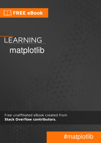
Imperative vs. Object-oriented SyntaxMatplotlib supports both object-oriented and imperative syntax for plotting. The imperative syntaxis intentionally designed to be very close to Matlab syntax.The imperative syntax (sometimes called 'state-machine' syntax) issues a string of commands allof which act on the most recent figure or axis (like Matlab). The object-oriented syntax, on theother hand, explicitly acts on the objects (figure, axis, etc.) of interest. A key point in the zen ofPython states that explicit is better than implicit so the object-oriented syntax is more pythonic.However, the imperative syntax is convenient for new converts from Matlab and for writing small,"throwaway" plot scripts. Below is an example of the two different styles.import matplotlib.pyplot as pltimport numpy as npt np.arange(0, 2, 0.01)y np.sin(4 * np.pi * t)# Imperative syntaxplt.figure(1)https://riptutorial.com/5
plt.clf()plt.plot(t, y)plt.xlabel('Time (s)')plt.ylabel('Amplitude (V)')plt.title('Sine Wave')plt.grid(True)# Object oriented syntaxfig plt.figure(2)fig.clf()ax fig.add subplot(1,1,1)ax.plot(t, y)ax.set xlabel('Time (s)')ax.set ylabel('Amplitude (V)')ax.set title('Sine Wave')ax.grid(True)Both examples produce the same plot which is shown below.Two dimensional (2D) arrayshttps://riptutorial.com/6
Display a two dimensional (2D) array on the axes.import numpy as npfrom matplotlib.pyplot import imshow, show, colorbarimage ad Getting started with matplotlib online: ngstarted-with-matplotlibhttps://riptutorial.com/7
Chapter 2: Animations and interactiveplottingIntroductionWith python matplotlib you can properly make animated graphs.ExamplesBasic animation with FuncAnimationThe matplotlib.animation package offer some classes for creating animations. FuncAnimationcreates animations by repeatedly calling a function. Here we use a function animate() that changesthe coordinates of a point on the graph of a sine function.import numpy as npimport matplotlib.pyplot as pltimport matplotlib.animation as animationTWOPI 2*np.pifig, ax plt.subplots()t np.arange(0.0, TWOPI, 0.001)s np.sin(t)l plt.plot(t, s)ax plt.axis([0,TWOPI,-1,1])redDot, plt.plot([0], [np.sin(0)], 'ro')def animate(i):redDot.set data(i, np.sin(i))return redDot,# create animation using the animate() functionmyAnimation animation.FuncAnimation(fig, animate, frames np.arange(0.0, TWOPI, 0.1), \interval 10, blit True, repeat True)plt.show()https://riptutorial.com/8
Save animation to gifIn this example we use the save method to save an Animation object using ImageMagick.import numpy as npimport matplotlib.pyplot as pltimport matplotlib.animation as animationfrom matplotlib import rcParams# make sure the full paths for ImageMagick and ffmpeg are configuredrcParams['animation.convert path'] r'C:\Program eg path'] r'C:\Program Files\ffmpeg\bin\ffmpeg.exe'TWOPI 2*np.pifig, ax plt.subplots()t np.arange(0.0, TWOPI, 0.001)s np.sin(t)l plt.plot(t, s)https://riptutorial.com/9
ax plt.axis([0,TWOPI,-1,1])redDot, plt.plot([0], [np.sin(0)], 'ro')def animate(i):redDot.set data(i, np.sin(i))return redDot,# create animation using the animate() function with no repeatmyAnimation animation.FuncAnimation(fig, animate, frames np.arange(0.0, TWOPI, 0.1), \interval 10, blit True, repeat False)# save animation at 30 frames per secondmyAnimation.save('myAnimation.gif', writer 'imagemagick', fps 30)Interactive controls with matplotlib.widgetsFor interacting with plots Matplotlib offers GUI neutral widgets. Widgets require amatplotlib.axes.Axes object.Here's a slider widget demo that ùpdates the amplitude of a sine curve. The update function istriggered by the slider's on changed() event.import numpy as npimport matplotlib.pyplot as pltimport matplotlib.animation as animationfrom matplotlib.widgets import SliderTWOPI 2*np.pifig, ax plt.subplots()t np.arange(0.0, TWOPI, 0.001)initial amp .5s initial amp*np.sin(t)l, plt.plot(t, s, lw 2)ax plt.axis([0,TWOPI,-1,1])axamp plt.axes([0.25, .03, 0.50, 0.02])# Slidersamp Slider(axamp, 'Amp', 0, 1, valinit initial amp)def update(val):# amp is the current value of the slideramp samp.val# update curvel.set ydata(amp*np.sin(t))# redraw canvas while idlefig.canvas.draw idle()# call update function on slider value changesamp.on 0
Other available widgets: lot live data from pipe with matplotlibhttps://riptutorial.com/11
This can be usefull when you want to visualize incoming data in real-time. This data could, forexample, come from a microcontroller that is continuously sampling an analog signal.In this example we will get our data from a named pipe (also known as a fifo). For this example,the data in the pipe should be numbers separted by newline characters, but you can adapt this toyour liking.Example data:100123.51589More information on named pipesWe will also be using the datatype deque, from the standard library collections. A deque objectworks quite a lot like a list. But with a deque object it is quite easy to append something to it whilestill keeping the deque object at a fixed length. This allows us to keep the x axis at a fixed lengthinstead of always growing and squishing the graph together. More information on deque objectsChoosing the right backend is vital for performance. Check what backends work on your operatingsystem, and choose a fast one. For me only qt4agg and the default backend worked, but thedefault one was too slow. More information on backends in matplotlibThis example is based on the matplotlib example of plotting random data.None of the ' characters in this code are meant to be removed.import matplotlibimport collections#selecting the right backend, change qt4agg to your desired backendmatplotlib.use('qt4agg')import matplotlib.pyplot as pltimport matplotlib.animation as animation#command to open the pipedatapipe open('path to your pipe','r')#amount of data to be displayed at once, this is the size of the x axis#increasing this amount also makes plotting slightly slowerdata amount 1000#set the size of the deque objectdatalist collections.deque([0]*data amount,data amount)#configure the graph itselffig, ax plt.subplots()line, ax.plot([0,]*data amount)#size of the y axis is set hereax.set ylim(0,256)def update(data):line.set ydata(data)return line,https://riptutorial.com/12
def data gen():while True:"""We read two data points in at once, to improve speedYou can read more at once to increase speedOr you can read just one at a time for improved animation smoothnessdata from the pipe comes in as a string,and is seperated with a newline character,which is why we use respectively eval and adline()).rstrip('\n')))yield datalistani animation.FuncAnimation(fig,update,data gen,interval 0, blit True)plt.show()If your plot starts to get delayed after a while, try adding more of the datalist.append data, so thatmore lines get read each frame. Or choose a faster backend if you can.This worked with 150hz data from a pipe on my 1.7ghz i3 4005u.Read Animations and interactive plotting utorial.com/13
Chapter 3: Basic PlotsExamplesScatter PlotsA simple scatter plotimport matplotlib.pyplot as plt# Datax 3,85]y 2,23]fig, ax plt.subplots(1, figsize (10, 6))fig.suptitle('Example Of Scatterplot')https://riptutorial.com/14
# Create the Scatter Plotax.scatter(x, y,color "blue",s 100,alpha 0.5,linewidths 1)####Color of the dotsSize of the dotsAlpha/transparency of the dots (1 is opaque, 0 is transparent)Size of edge around the dots# Show the plotplt.show()A Scatterplot with Labelled Pointsimport matplotlib.pyplot as plt# Datax [21, 34, 44, 23]y [435, 334, 656, 1999]labels ["alice", "bob", "charlie", "diane"]# Create the figure and axes objectshttps://riptutorial.com/15
fig, ax plt.subplots(1, figsize (10, 6))fig.suptitle('Example Of Labelled Scatterpoints')# Plot the scatter pointsax.scatter(x, y,color "blue",s 100,alpha 0.5,linewidths 1)####Color of the dotsSize of the dotsAlpha of the dotsSize of edge around the dots# Add the participant names as text labels for each pointfor x pos, y pos, label in zip(x, y, labels):ax.annotate(label,# The label for this pointxy (x pos, y pos), # Position of the corresponding pointxytext (7, 0),# Offset text by 7 points to the righttextcoords 'offset points', # tell it to use offset pointsha 'left',# Horizontally aligned to the leftva 'center')# Vertical alignment is centered# Show the plotplt.show()Shaded PlotsShaded region below a linehttps://riptutorial.com/16
import matplotlib.pyplot as plt# Datax [0,1,2,3,4,5,6,7,8,9]y1 [10,20,40,55,58,55,50,40,20,10]# Shade the area between y1 and lineplt.fill between(x, y1, 0,facecolor "orange",color 'blue',alpha 0.2)y 0# The fill color# The outline color# Transparency of the fill# Show the plotplt.show()Shaded Region between two lineshttps://riptutorial.com/17
import matplotlib.pyplot as plt# Datax [0,1,2,3,4,5,6,7,8,9]y1 [10,20,40,55,58,55,50,40,20,10]y2 [20,30,50,77,82,77,75,68,65,60]# Shade the area between y1 and y2plt.fill between(x, y1, y2,facecolor "orange", # The fill colorcolor 'blue',# The outline coloralpha 0.2)# Transparency of the fill# Show the plotplt.show()Line plotsSimple line plothttps://riptutorial.com/18
import matplotlib.pyplot as plt# Datax 7,95]y 2,23]# Create the plotplt.plot(x, y, 'r-')# r- is a style code meaning red solid line# Show the plotplt.show()Note that in general y is not a function of x and also that the values in x do not need to be sorted.Here's how a line plot with unsorted x-values looks like:# shuffle the elements in xnp.random.shuffle(x)plt.plot(x, y, 'r-')plt.show()https://riptutorial.com/19
Data plotThis is similar to a scatter plot, but uses the plot() function instead. The only difference in thecode here is the style argument.plt.plot(x, y, 'b ')# Create blue up-facing triangleshttps://riptutorial.com/20
Data and lineThe style argument can take symbols for both markers and line style:plt.plot(x, y, 'go--')# green circles and dashed linehttps://riptutorial.com/21
HeatmapHeatmaps are useful for visualizing scalar functions of two variables. They provide a “flat” image oftwo-dimensional histograms (representing for instance the density of a certain area).The following source code illustrates heatmaps using bivariate normally distributed numberscentered at 0 in both directions (means [0.0, 0.0]) and a with a given covariance matrix. The datais generated using the numpy function numpy.random.multivariate normal; it is then fed to thehist2d function of pyplot 2
import numpy as npimport matplotlibimport matplotlib.pyplot as plt# Define numbers of generated data points and bins per axis.N numbers 100000N bins 100# set random seednp.random.seed(0)# Generate 2D normally distributed numbers.x, y np.random.multivariate normal(mean [0.0, 0.0],# meancov [[1.0, 0.4],[0.4, 0.25]],# covariance matrixsize N numbers).T# transpose to get columns# Construct 2D histogram from data using the 'plasma' colormapplt.hist2d(x, y, bins N bins, normed False, cmap 'plasma')https://riptutorial.com/23
# Plot a colorbar with label.cb plt.colorbar()cb.set label('Number of entries')# Add title and labels to plot.plt.title('Heatmap of 2D normally distributed data points')plt.xlabel('x axis')plt.ylabel('y axis')# Show the plot.plt.show()Here is the same data visualized as a 3D histogram (here we use only 20 bins for efficiency). Thecode is based on this matplotlib demo.from mpl toolkits.mplot3d import Axes3Dimport numpy as npimport matplotlibimport matplotlib.pyplot as plt# Define numbers of generated data points and bins per axis.https://riptutorial.com/24
N numbers 100000N bins 20# set random seednp.random.seed(0)# Generate 2D normally distributed numbers.x, y np.random.multivariate normal(mean [0.0, 0.0],# meancov [[1.0, 0.4],[0.4, 0.25]],# covariance matrixsize N numbers).T# transpose to get columnsfig plt.figure()ax fig.add subplot(111, projection '3d')hist, xedges, yedges np.histogram2d(x, y, bins N bins)# Add title and labels to plot.plt.title('3D histogram of 2D normally distributed data points')plt.xlabel('x axis')plt.ylabel('y axis')# Construct arrays for the anchor positions of the bars.# Note: np.meshgrid gives arrays in (ny, nx) so we use 'F' to flatten xpos,# ypos in column-major order. For numpy 1.7, we could instead call meshgrid# with indexing 'ij'.xpos, ypos np.meshgrid(xedges[:-1] 0.25, yedges[:-1] 0.25)xpos xpos.flatten('F')ypos ypos.flatten('F')zpos np.zeros like(xpos)# Construct arrays with the dimensions for the 16 bars.dx 0.5 * np.ones like(zpos)dy dx.copy()dz hist.flatten()ax.bar3d(xpos, ypos, zpos, dx, dy, dz, color 'b', zsort 'average')# Show the plot.plt.show()Read Basic Plots online: c-plotshttps://riptutorial.com/25
Chapter 4: BoxplotsExamplesBasic BoxplotsBoxplots are descriptive diagrams that help to compare the distribution of different series of data.They are descriptive because they show measures (e.g. the median) which do not assume anunderlying probability distribution.The most basic example of a boxplot in matplotlib can be achieved by just passing the data as alist of lists:import matplotlib as pltdataline1 3,85]dataline2 2,23]data [ dataline1, dataline2 ]plt.boxplot( data )However, it is a common practice to use numpy arrays as parameters to the plots, since they areoften the result of previous calculations. This can be done as follows:import numpy as npimport matplotlib as pltnp.random.seed(123)dataline1 np.random.normal( loc 50, scale 20, size 18 )dataline2 np.random.normal( loc 30, scale 10, size 18 )data np.stack( [ dataline1, dataline2 ], axis 1 )plt.boxplot( data )https://riptutorial.com/26
Read Boxplots online: lotshttps://riptutorial.com/27
Chapter 5: BoxplotsExamplesBoxplot functionMatplotlib has its own implementation of boxplot. The relevant aspects of this function is that, bydefault, the boxplot is showing the median (percentile 50%) with a red line. The box represents Q1and Q3 (percentiles 25 and 75), and the whiskers give an idea of the range of the data (possibly atQ1 - 1.5IQR; Q3 1.5IQR; being IQR the interquartile range, but this lacks confirmation). Alsonotice that samples beyond this range are shown as markers (these are named fliers).NOTE: Not all implementations of boxplot follow the same rules. Perhaps the mostcommon boxplot diagram uses the whiskers to represent the minimum and maximum(making fliers non-existent). Also notice that this plot is sometimes called box-andwhisker plot and box-and-whisker diagram.The following recipe show some of the things you can do with the current matplotlibimplementation of boxplot:import matplotlib.pyplot as pltimport numpy as npX1 np.random.normal(0, 1, 500)X2 np.random.normal(0.3, 1, 500)# The most simple boxplotplt.boxplot(X1)plt.show()# Changing some of its featuresplt.boxplot(X1, notch True, sym "o") # Use sym "" to shown no fliers; also showfliers Falseplt.show()# Showing multiple boxplots on the same windowplt.boxplot((X1, X2), notch True, sym "o", labels ["Set 1", "Set 2"])plt.show()# Hidding features of the boxplotplt.boxplot(X2, notch False, showfliers False, showbox False, showcaps False, positions [4],labels ["Set 2"])plt.show()# Advanced customization of the boxplotline props dict(color "r", alpha 0.3)bbox props dict(color "g", alpha 0.9, linestyle "dashdot")flier props dict(marker "o", markersize 17)plt.boxplot(X1, notch True, whiskerprops line props, boxprops bbox props,flierprops flier props)plt.show()This result in the following plots:https://riptutorial.com/28
1. Default matplotlib boxplothttps://riptutorial.com/29
2. Changing some features of the boxplot using function argumentshttps://riptutorial.com/30
3. Multiple boxplot in the same plot windowhttps://riptutorial.com/31
4. Hidding some features of the boxplothttps://riptutorial.com/32
5. Advanced customization of a boxplot using propsIf you intend to do some advanced customization of your boxplot you should know that the propsdictionaries you build (for example):line props dict(color "r", alpha 0.3)bbox props dict(color "g", alpha 0.9, linestyle "dashdot")flier props dict(marker "o", markersize 17)plt.boxplot(X1, notch True, whiskerprops line props, boxprops bbox props,flierprops flier props)plt.show().refer mostly (if not all) to Line2D objects. This means that only arguments available in that classare changeable. You will notice the existence of keywords such as whiskerprops, boxprops,flierprops, and capprops. These are the elements you need to provide a props dictionary to furthercustomize it.NOTE: Further customization of the boxplot using this implementation might provedifficult. In some instances the use of other matplotlib elements such as patches tohttps://riptutorial.com/33
build ones own boxplot can be advantageous (considerable changes to the boxelement, for example).Read Boxplots online: lotshttps://riptutorial.com/34
Chapter 6: Closing a figure windowSyntax plt.close() # closes the current active figureplt.close(fig) # closes the figure with handle 'fig'plt.close(num) # closes the figure number 'num'plt.close(name) # closes the figure with the label 'name'plt.close('all') # closes all figuresExamplesClosing the current active figure using pyplotThe pyplot interface to matplotlib might be the simplest way to close a figure.import matplotlib.pyplot as pltplt.plot([0, 1], [0, 1])plt.close()Closing a specific figure using plt.close()A specific figure can be closed by keeping its handleimport matplotlib.pyplot as pltfig1 plt.figure() # create first figureplt.plot([0, 1], [0, 1])fig2 plt.figure() # create second figureplt.plot([0, 1], [0, 1])plt.close(fig1) # close first figure although second one is activeRead Closing a figure window online: ing-a-figurewindowhttps://riptutorial.com/35
Chapter 7: ColormapsExamplesBasic usageUsing built-in colormaps is as simple as passing the name of the required colormap (as given inthe colormaps reference) to the plotting function (such as pcolormesh or contourf) that expects it,usually in the form of a cmap keyword argument:import matplotlib.pyplot as pltimport numpy as ,cmap 'hot')plt.show()https://riptutorial.com/36
Colormaps are especially useful for visualizing three-dimensional data on two-dimensional plots,but a good colormap can also make a proper three-dimensional plot much clearer:import matplotlib.pyplot as pltfrom mpl toolkits.mplot3d import Axes3Dfrom matplotlib.ticker import LinearLocator# generate example dataimport numpy as npx,y 15))z np.cos(x*np.pi)*np.sin(y*np.pi)# actual plotting examplefig plt.figure()ax1 fig.add subplot(121, projection '3d')ax1.plot surface(x,y,z,rstride 1,cstride 1,cmap 'viridis')ax2 fig.add subplot(122)cf ax2.contourf(x,y,z,51,vmin -1,vmax 1,cmap 'viridis')cbar fig.colorbar(cf)cbar.locator LinearLocator(numticks 11)cbar.update ticks()for ax in {ax1, ax2}:ax.set xlabel(r' x ')ax.set ylabel(r' y ')ax.set xlim([-1,1])ax.set ylim([-1,1])ax.set aspect('equal')ax1.set zlim([-1,1])ax1.set zlabel(r' \cos(\pi x) \sin(\pi y) ')plt.show()https://riptutorial.com/37
Using custom colormapsApart from the built-in colormaps defined in the colormaps reference (and their reversed maps,with ' r' appended to their name), custom colormaps can also be defined. The key is thematplotlib.cm module.The below example defines a very simple colormap using cm.register cmap, containing a singlecolour, with the opacity (alpha value) of the colour interpolating between fully opaque and fullytransparent in the data range. Note that the important lines from the point of view of the colormapare the import of cm, the call to register cmap, and the passing of the colormap to plot surface.import matplotlib.pyplot as pltfrom mpl toolkits.mplot3d import Axes3Dimport matplotlib.cm as cm# generate data for spherefrom numpy import pi,meshgrid,linspace,sin,costh,ph ,z tutorial.com/38
# define custom colormap with fixed colour and alpha gradient# use simple linear interpolation in the entire scalecm.register cmap(name 'alpha gradient',data {'red':[(0.,0,0),(1.,0,0)],'green': 1.,0.4,0.4)],'alpha': [(0.,1,1),(1.,0,0)]})# plot sphere with custom colormap; constrain mapping to between z 0.7 for enhanced effectfig plt.figure()ax fig.add subplot(111, projection '3d')ax.plot surface(x,y,z,cmap 'alpha gradient',vmin 0.7,vmax 0.7,rstride 1,cstride 1,linewidth 0.5,edgecolor 'b')ax.set xlim([-1,1])ax.set ylim([-1,1])ax.set zlim([-1,1])ax.set 9
In more complicated scenarios, one can define a list of R/G/B(/A) values into which matplotlibinterpolates linearly in order to determine the colours used in the corresponding plots.Perceptually uniform colormapsThe original default colourmap of MATLAB (replaced in version R2014b) called jet is ubiquitousdue to its high contrast and familiarity (and was the default of matplotlib for compatibility reasons).Despite its popularity, traditional colormaps often have deficiencies when it comes to representingdata accurately. The percieved change in these colormaps does not correspond to changes indata; and a conversion of the colormap to greyscale (by, for instance, printing a figure using ablack-and-white printer) might cause loss of information.Perceptually uniform colormaps have been introduced to make data visualization as accurate andaccessible as possible. Matplotlib introduced four new, perceptually uniform colormaps in version1.5, with one of them (named viridis) to be the default from version 2.0. These four colormaps (viridis, inferno, plasma and magma) are all optimal from the point of view of perception, and theseshould be used for data visualization by default unless there are very good reasons not to do so.These colormaps introduce as little bias as possible (by not creating features where there aren'thttps://riptutorial.com/40
any to begin with), and they are suitable for an audience with reduced color perception.As an example for visually distorting data, consider the following two top-view plots of pyramid-likeobjects:Which one of the two is a proper pyramid? The answer is of course that both of them are, but thisis far from obvious from the plot using the jet colormap:https://riptutorial.com/41
This feature is at the core of perceptual uniformity.Custom discrete colormapIf you have predefined ranges and want to use specific colors for those ranges you can declarecustom colormap. For example:import matplotlib.pyplot as pltimport num
The matplotlib.animation package offer some classes for creating animations. FuncAnimation creates animations by repeatedly calling a function. Here we use a function animate() that changes the coordinates of a point on the graph of a sine function. import numpy as np import matplotlib.pyplot as plt import matplotlib