Transcription
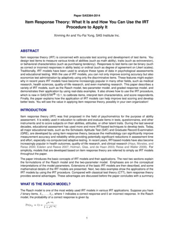
Paper SAS364-2014Item Response Theory: What It Is and How You Can Use the IRTProcedure to Apply ItXinming An and Yiu-Fai Yung, SAS Institute Inc.ABSTRACTItem response theory (IRT) is concerned with accurate test scoring and development of test items. Youdesign test items to measure various kinds of abilities (such as math ability), traits (such as extroversion),or behavioral characteristics (such as purchasing tendency). Responses to test items can be binary (suchas correct or incorrect responses in ability tests) or ordinal (such as degree of agreement on Likert scales).Traditionally, IRT models have been used to analyze these types of data in psychological assessmentsand educational testing. With the use of IRT models, you can not only improve scoring accuracy but alsoeconomize test administration by adaptively using only the discriminative items. These features might explainwhy in recent years IRT models have become increasingly popular in many other fields, such as medicalresearch, health sciences, quality-of-life research, and even marketing research. This paper describes avariety of IRT models, such as the Rasch model, two-parameter model, and graded response model, anddemonstrates their application by using real-data examples. It also shows how to use the IRT procedure,which is new in SAS/STAT 13.1, to calibrate items, interpret item characteristics, and score respondents.Finally, the paper explains how the application of IRT models can help improve test scoring and developbetter tests. You will see the value in applying item response theory, possibly in your own organization!INTRODUCTIONItem response theory (IRT) was first proposed in the field of psychometrics for the purpose of abilityassessment. It is widely used in education to calibrate and evaluate items in tests, questionnaires, and otherinstruments and to score subjects on their abilities, attitudes, or other latent traits. During the last severaldecades, educational assessment has used more and more IRT-based techniques to develop tests. Today,all major educational tests, such as the Scholastic Aptitude Test (SAT) and Graduate Record Examination(GRE), are developed by using item response theory, because the methodology can significantly improvemeasurement accuracy and reliability while providing potentially significant reductions in assessment timeand effort, especially via computerized adaptive testing. In recent years, IRT-based models have also becomeincreasingly popular in health outcomes, quality-of-life research, and clinical research (Hays, Morales, andReise 2000; Edelen and Reeve 2007; Holman, Glas, and de Haan 2003; Reise and Waller 2009). Forsimplicity, models that are developed based on item response theory are referred to simply as IRT modelsthroughout the paper.The paper introduces the basic concepts of IRT models and their applications. The next two sections explainthe formulations of the Rasch model and the two-parameter model. Emphases are on the conceptualinterpretations of the model parameters. Extensions of the basic IRT models are then described, and somemathematical details of the IRT models are presented. Next, two data examples show the applications of theIRT models by using the IRT procedure. Compared with classical test theory (CTT), item response theoryprovides several advantages. These advantages are discussed before the paper concludes with a summary.WHAT IS THE RASCH MODEL?The Rasch model is one of the most widely used IRT models in various IRT applications. Suppose you haveJ binary items, X1 ; : : : ; XJ , where 1 indicates a correct response and 0 an incorrect response. In the Raschmodel, the probability of a correct response is given byPr.xij D 1/ De i j1 C e i j1
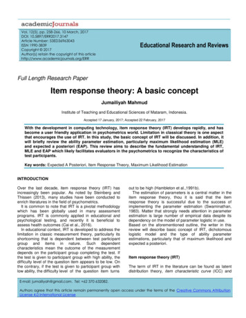
where i is the ability (latent trait) of subject i and j is the difficulty parameter of item j. The probability ofa correct response is determined by the item’s difficulty and the subject’s ability. This probability can beillustrated by the curve in Figure 1, which is called the item characteristic curve (ICC) in the field of IRT. Fromthis curve you can observe that the probability is a monotonically increasing function of ability. This meansthat as the subject’s ability increases, the probability of a correct response increases; this is what you wouldexpect in practice.Figure 1 Item Characteristic CurveAs the name suggests, the item difficulty parameter measures the difficulty of answering the item correctly.The preceding equation suggests that the probability of a correct response is 0.5 for any subject whoseability is equal to the value of the difficulty parameter. Figure 2 shows the ICCs for three items, with difficultyparameters of –2, 0, and 2. By comparing these three ICCs, you can see that the location of the ICC isdetermined by the difficulty parameter. To get a 0.5 probability of a correct response for these three items,the subject must have an ability of –2, 0, and 2, respectively.Figure 2 Item Characteristic Curves2
WHAT IS THE TWO-PARAMETER MODEL?In the Rasch model, all the items are assumed to have the same shape. In practice, however, this assumptionmight not be reasonable. To avoid this assumption, another parameter called the discrimination (slope)parameter is introduced. The resulting model is called the two-parameter model. In the two-parametermodel, the probability of a correct response is given byPr.Xij D 1/ De j i j1 C e j i jwhere j is the discrimination parameter for item j. The discrimination parameter is a measure of thedifferential capability of an item. A high discrimination parameter value suggests an item that has a highability to differentiate subjects. In practice, a high discrimination parameter value means that the probability ofa correct response increases more rapidly as the ability (latent trait) increases. Item characteristic curves ofthree items, item1, item2, and item3, with different discrimination parameter values are shown in Figure 3.Figure 3 Item Characteristic CurvesThe difficulty parameter values for these three items are all 0. The discrimination parameter values are 0.3,1, and 2, respectively. In Figure 3, you can observe that as the discrimination parameter value increases, theICC becomes more steep around 0. As the ability value changes from –0.5 to 0.5, the probability of a correctresponse changes from 0.3 to 0.7 for item3, which is much larger than item1. For that reason, item3 candifferentiate subjects whose ability value is around 0 more efficiently than item1 can.EXTENSIONS OF THE BASIC IRT MODELSEarly IRT models, such as the Rasch model and the two-parameter model, concentrate mainly on analyzingdichotomous responses that have a single latent trait. The preceding sections describe the characteristics ofthese two models. Various extensions of these basic IRT models have been developed for more flexiblemodeling in different situations. The following list presents some extended (or generalized) IRT models andtheir capabilities: graded response models (GRM), which analyze ordinal responses and rating scales three- and four-parameter models, which analyze test items that have guessing and ceiling parametersin the response curves3
multidimensional IRT models, which analyze test items that can be explained by more than one latenttrait or factor multiple-group IRT models, which analyze test items in independent groups to study differential itemfunctioning or invariance confirmatory IRT models, which analyze test items that have hypothesized relationships with the latentfactorsThese generalizations or extensions of IRT models are not mutually exclusive. They can be combined toaddress the complexity of the data and to test the substantive theory in practical applications. Althoughthe IRT procedure handles most of these complex models, it is beyond the scope of this paper to describeall these models in detail. For general references about various IRT models, see De Ayala (2009) andEmbretson and Reise (2000). The current paper focuses on the basic unidimensional IRT models that areused in the majority of applications.SOME MATHEMATICAL DETAILS OF IRT MODELSThis section provides mathematical details of the multidimensional graded response model for ordinal items.This model subsumes most basic IRT models, such as the Rasch model and the two-parameter model, asspecial cases. Mathematically inclined readers might find this section informative, whereas others mightprefer to skip it if their primary goal is practical applications.A d-dimensional IRT model that has J ordinal responses can be expressed by the equationsyij D j i C ijpij k D Pr.uij D k/ D Pr. .j;k1/k D 1; : : : ; K yij .j;k/ /;where uij is the observed ordinal response from subject i for item j; yij is a continuous latent responsethat underlies uij ; j D . .j;0/ D 1; .j;1/ ; : : : ; .j;K 1/ ; .j;K/ D 1/ is a vector of threshold parameters foritem j; j is a vector of slope (or discrimination) parameters for item j; i D . i1 ; : : : ; id / is a vector of latentfactors for subject i, i Nd . ; †/; and i D . i1 ; : : : ; iJ / is a vector of unique factors for subject i. Allthe unique factors in i are independent of one another, suggesting that yij ; j D 1; : : : ; J , are independentconditional on the latent factor i . (This is the so-called local independence assumption.) Finally, i and iare also independent.Based on the preceding model specification,Z .j;k/Zpij k D .j;k/ j ip.yI j i ; 1/dy D .j;k1/p.yI 0; 1/dy .j;k1/ j iwhere p is determined by the link function. It is the density function of the standard normal distribution if theprobit link is used, or the density function of the logistic distribution if the logistic link is used.The model that is specified in the preceding equation is called the multidimensional graded response model.When the responses are binary and there is only one latent factor, this model reduces to the two-parametermodel, which can be expressed asyij D j i C ijpij D Pr.uij D 1/ D Pr.yij j /A different parameterization for the two-parameter model isyij D aj . ibj / C ijpij D Pr.uij D 1/ D Pr.yij 0/where bj is interpreted as item difficulty and aj is called the discrimination parameter. The preceding twoparameterizations are mathematically equivalent. For binary response items, you can transfer the threshold parameter into the difficulty parameter by bj D jj . The IRT procedure uses the first parameterization.4
The two-parameter model reduces to a one-parameter model when slope parameters for all the items areconstrained to be equal. In the case where the logistic link is used, the one- and two-parameter models areoften abbreviated as 1PL and 2PL, respectively. When all the slope parameters are set to 1 and the factorvariance is set to a free parameter, you obtain the Rasch model.You can obtain three- and four-parameter models by introducing the guessing and ceiling parameters. Letgj and cj denote the item-specific guessing and ceiling parameters, respectively. Then the four-parametermodel can be expressed aspij D Pr.uij D 1/ D gj C .cjgj / Pr.yij 0/This model reduces to the three-parameter model when cj D 1.EXAMPLE 1: LAW SCHOOL ADMISSION TESTThe data set in this example comes from the Law School Admission Test (LSAT). It includes the responsesof 1,000 subjects to five binary items. The following DATA step creates the data set IrtLsat:data IrtLsat;input item1-item5 @@;datalines;0 0 0 0 0. more lines .1 1 1 1 1;The following statements fit the IRT model by using all the default settings. The PLOTS option is used torequest the scree plot and the item characteristic curves, with the arguments SCREE and ICC.ods graphics on;proc irt data IrtLsat plots (scree icc);var item1-item5;run;The unidimensional assumption suggests that the correlation among these items can be explained by asingle latent factor. You can check this assumption by examining the eigenvalues and the magnitude ofthe item slope (discrimination) parameters. A small slope parameter value (such as 0.5) often suggeststhat the corresponding item is not a good indicator of the latent construct. Figure 4 and Figure 5 show theeigenvalue table and the scree plot, respectively. You can see that the first eigenvalue is much greater thanthe others, suggesting that a unidimensional model is reasonable for this example.Figure 4 Eigenvalues of Polychoric CorrelationsThe IRT ProcedureEigenvalues of the Polychoric Correlation MatrixEigenvalue Difference Proportion Cumulative1 1.95547526 0.970647930.39110.39112 0.98482733 0.127847020.19700.58813 0.85698031 0.120098700.17140.75954 0.73688161 0.271046120.14740.90685 0.465835490.09321.00005
Figure 5 Scree PlotsParameter estimates for this example are shown in Figure 6. Under the parameterization used by PROCIRT, the slope parameter is the same as the discrimination parameter. As a result, these parameters areused interchangeably throughout this paper. The threshold parameter has the same interpretation as thedifficulty parameter. For this example, the threshold parameter estimates range from –2.59 to –0.19; item1is the easiest item, and item3 is the most difficult item. The fact that all the threshold parameter estimatesare less than 0 suggests that all the items in this example are relatively easy and therefore are most usefulin discriminating subjects who have lower abilities. As mentioned in the preceding section, the thresholdparameter can be transformed into the difficulty parameter. For each ICC plot shown in Figure 7, the verticalreference line indicates the difficulty of each item. The difficulty parameter value is shown at the top of eachplot beside the vertical reference line.The slope parameter values for this example range from 0.45 to 1.36. By comparing the ICCs in Figure 7,you can observe how the value of the slope parameter affects the shape of the ICC. Among these five items,the ICC for item1 is the steepest and the ICC for item3 is the flattest.Figure 6 Parameter EstimatesThe IRT ProcedureItem Parameter EstimatesParameter EstimateStandardError Pr t item1 Threshold -2.590870.22115 .0001ItemSlope1.362250.25067 .0001item2 Threshold -1.058590.12506 .0001Slope1.323880.27282 .0001item3 Threshold -0.193130.06667 0.0019Slope0.448450.11478 .0001item4 Threshold -1.264960.10733 .0001Slope0.952890.18798 .0001item5 Threshold -1.981400.12915 .0001Slope0.8266560.17174 .0001
Figure 7 Item Characteristic CurvesEXAMPLE 2: QUALITY OF LIFE SURVEYThe data set in this example comes from the 1978 Quality of American Life Survey. The survey wasadministered to a sample of all US residents aged 18 years and older in 1978. Subjects were asked to ratetheir satisfaction with many different aspects of their lives. This example includes 14 items. Some of theitems are as follows: satisfaction with community satisfaction with neighbors satisfaction with amount of education received satisfaction with health satisfaction with job satisfaction with incomeThis example uses 1,000 random samples from the original data set. The following DATA step creates thedata set IrtSat:data IrtSat;input item1-item14 @@;datalines;11211222.2222222.11113. more lines .111122;For illustration purposes, these items are reorganized into different numbers of categories. The number ofcategories ranges from 2 to 7. By default, the IRT procedure uses the graded response model (GRM) withthe logistic link for all the items. For binary response, the GRM is equivalent to the two-parameter model. In7
PROC IRT, you can specify different types of response models for different items by using the RESFUNC option in the MODEL statement.For this example, because all the items are designed to measure subjects’ satisfaction with different aspectsof their lives, it is reasonable to start with a unidimensional IRT model. The following statements fit such amodel by using all the default options:ods graphics on;proc irt data IrtSat plots (iic tic) ;var item1-item14;run;Figure 8 shows the eigenvalue table for this example. You can see that the first eigenvalue is much greaterthan the others, suggesting that a unidimensional model is reasonable for this example.Figure 8 Eigenvalues of Polychoric CorrelationsThe IRT ProcedureEigenvalues of the Polychoric Correlation MatrixEigenvalue Difference Proportion Cumulative1 5.57173396 4.196146140.39800.39802 1.37558781 0.292732440.09830.49623 1.08285537 0.126000330.07730.57364 0.95685504 0.091089090.06830.64195 0.86576595 0.097582210.06180.70386 0.76818374 0.125716830.05490.75867 0.64246691 0.061083050.04590.80458 0.58138386 0.042145530.04150.84619 0.53923833 0.100928350.03850.884610 0.43830998 0.073469770.03130.915911 0.36484021 0.046679350.02610.941912 0.31816085 0.039051350.02270.964713 0.27910950 0.063601010.01990.984614 0.215508490.01541.0000In the context of IRT, the amount of information that each item or test provides is not evenly distributedacross the entire continuum of latent constructs. The value of the slope parameter represents the amountof information provided by the item. For this example, parameter estimates and item information curvesare shown in Figure 9 and Figure 10, respectively. By examining the parameter estimates and the iteminformation curves, you can see that items that have high slope values are more informative than items thathave low slope values. For example, because the slope value of item1 is much smaller than the slope valueof item9, the information curve is flatter for item1 than for item9.For individual items, most of the information concentrates around the area defined by the threshold parameters. The binary response item provides most of the information around the threshold. For ordinal items,most of the information falls in the range defined by the lowest and the highest threshold parameters. Bycomparing the information curves for item7 and item9, you can also see that in cases where response itemshave the same slope value, the ordinal item is more informative than the binary item.Item selection is an important process for test (questionnaire) development. It serves two purposes: toensure that all the items included in the test are sufficiently unidimensional, and to maximize the testinformation across the interested continuum of latent constructs. During the item selection process, ideallyyou want to select high-differential items whose threshold parameters cover the interested latent constructcontinuum. However, in practice you often encounter the situation in which these high-differential itemscannot provide enough information for the entire continuum, especially when these items are binary. In thissituation, you might need to select some lower-differential items that can add information to the area that isnot covered by these high-differential items.8
Figure 9 Parameter EstimatesThe IRT ProcedureItem Parameter EstimatesItemParameterEstimateStandardError Pr t item1Threshold 1 -0.955030.07367 .0001Threshold 21.479240.08372 .0001Slope0.453940.07042 .0001Threshold 1 -0.655310.08328 .0001Threshold 20.568980.08242 .0001Slope1.206470.09708 .0001Threshold0.001700.07114 0.4905Slope0.724280.08511 .0001-0.441550.08367 .236500.11147 .0001Threshold 1 -0.738370.08045 .0001Threshold 20.641130.07930 .0001Slope1.038100.08755 .0001Threshold 1 -0.422520.07133 .0001Threshold 20.851630.07544 .0001Slope0.707860.07605 .0001Threshold 1 -1.471660.11278 .0001The IRT ProcedureItem Parameter EstimatesEstimateStandardError Pr t Threshold 20.484140.10006 .0001Threshold 31.689360.11665 .0001Slope1.893610.12255 .0001Threshold 1 -1.044830.09261 .0001Threshold 20.877770.09072 .0001Threshold 31.947150.11031 .0001Slope1.412420.09836 .0001Threshold0.334400.11941 0.0026Slope1.850670.20122 .0001item10 Threshold 1 -0.544240.09447 .0001Itemitem8item9ParameterThreshold 21.159230.10220 .0001Slope1.669430.12080 .0001item11 Threshold 1 -1.699190.11397 .0001Threshold 2 -0.035510.09403 0.3529Threshold 31.097600.10224 .0001Threshold 42.274040.12716 .0001Slope1.661350.10896 .00019
Figure 9 continuedThe IRT ProcedureItem Parameter EstimatesEstimateStandardError Pr t item12 Threshold 1 -2.226870.11781 .0001Threshold 2 -0.950570.08845 .0001Threshold 3 -0.101650.08221 0.1082Threshold 40.732780.08572 .0001Threshold 51.485100.09659 .0001Threshold 62.208420.11444 .0001Slope1.188610.08590 .0001item13 Threshold 1 -1.998080.14409 .0001ItemParameterThreshold 20.818780.12153 .0001Threshold 32.729390.16482 .0001Slope2.477420.15809 .0001item14 Threshold 1 -1.901890.10988 .0001Threshold 20.513780.08654 .0001Threshold 31.918700.10854 .0001Slope1.391190.09549 .0001Figure 10 Item Information Curves10
Figure 10 continued11
For this example, the slope parameters range from 0.45 to 2.47, and the threshold parameters range from–2.23 to 2.47. Among these 14 items, three of them, item1, item3, and item6, have slope values below 1,and the slope value for item1 is below 0.5. The item information curves suggest that these three items,especially item1, provide much less information than the other items. As a result, you might considerdropping these three items. Figure 11 shows the test information curves for the original test that has 14items and the shorter test that excludes item1, item3, and item6. The two information curves are almostidentical, suggesting that the shorter test provides almost the same amount of information as the longer test.After item calibration and item selection, another important task is to score subjects based on their responses.In IRT, there are three widely used scoring methods: maximum likelihood (ML), maximum a posteriori (MAP),and expected a posteriori (EAP). You can specify them by using the SCOREMETHOD option in the PROCIRT statement. The following example code scores the subject based on the shorter test by using the MAPmethod:proc irt data IrtSat scoremethod map;var item2 item4 item5 item7-item14;run;Figure 11 Test Information CurvesITEM RESPONSE THEORY—DOES IT OFFER MORE THAN CTT CAN PROVIDE?Classic test theory (CTT) has been the basis for developing psychological scales and test scoring for manydecades. You might wonder why you would need IRT models, which serve similar purposes. This sectionpoints out some conceptual and practical advantages of IRT models over CTT models in regard to test orscale construction and development. The main purpose is to point out that IRT models have unique featuresthat complement CTT-based measures rather than to thoroughly compare the two approaches.First, a limitation of CTT is that the item and person characteristics, such as item difficulty parameters andperson scores, are not discernible. Depending on the subpopulation in question, item characteristics mightchange. If a high-ability subpopulation is considered, all test items would appear to be easy. But when a12
low-ability subpopulation is considered, the same set of items would be difficult. This limitation makes itdifficult to assess individuals’ abilities by using different test forms. However, in IRT, the item characteristicsand the personal abilities are formulated by distinctive parameters. After the items are calibrated for apopulation, the scores for subjects from that population can be compared directly even if they answer differentsubsets of the items. Some researchers refer to this as the invariant property of IRT models (for example,see Hambleton, Swaminathan, and Rogers 1991).Second, the definition of reliability in CTT is based on parallel tests, which are difficult to achieve in practice.The precision of measurement is the same for all scores for a particular sample. In CTT, longer tests areusually more reliable than shorter tests. However, reliability in IRT is defined as a function that is conditionalon the scores of the measured latent construct. Precision of measurement differs across the latent constructcontinuum and can be generalized to the whole target population. In IRT, measurement precision is oftendepicted by the information curves. These curves can be treated as a function of the latent factor conditionalon the item parameters. They can be calculated for an individual item (item information curve) or for thewhole test (test information curve). The test information curve can be used to evaluate the performance ofthe test. During test development, you want to make sure that the selected items can provide adequateprecision across the interested range of the latent construct continuum.Third, missing values in CTT are difficult to handle during both test development and subject scoring.Subjects who have one or more missing responses cannot be scored unless these missing values areimputed. In contrast, the estimation framework of IRT models makes it straightforward to analyze itemsthat have random missing data. IRT can still calibrate items and score subjects by using all the availableinformation based on the likelihood; the likelihood-based methods are implemented in the IRT procedure.MAIN FEATURES OF THE IRT PROCEDUREThe IRT procedure enables you to estimate various IRT models. The following list summarizes some of themain features of PROC IRT: fits the following classes of models: Rasch model; one-, two-, three-, and four-parameter models; andgraded response models supports logistic and probit links calibrates items that can have different response models performs multidimensional exploratory and confirmatory analysis performs multiple-group analysis, with fixed values and equality constraints within and between groups estimates factor scores by using the maximum likelihood (ML), maximum a posteriori (MAP), orexpected a posteriori (EAP) method supports the quasi-Newton (QN) and expectation-maximization (EM) algorithms for optimizationSUMMARYThis paper provides a brief introduction to item response theory (IRT) and the related models. The Raschand two-parameter models are the two models most frequently used in applications. Basic concepts andinterpretations of these basic models are described. Examples illustrate the use of the IRT procedure,which is new in SAS/STAT 13.1, for fitting IRT models and selecting useful items. IRT provides a modelingframework that you can use to study item characteristics and person scores unambiguously from the data.Some advantages of IRT over classic testing theory (CTT) are discussed. The data examples in this paperillustrate only some of the functionality that PROC IRT provides. Actual test developments might requiremore extensive analysis, including measures based on CTT and inputs from content experts. For detaileddiscussions of test development, see DeVellis (2011) and Edelen and Reeve (2007).13
REFERENCESDe Ayala, R. J. (2009), The Theory and Practice of Item Response Theory, New York: Guilford Press.DeVellis, R. F. (2011), Scale Development: Theory and Applications, 3rd Edition, Thousand Oaks, CA: SagePublications.Edelen, M. O. and Reeve, B. B. (2007), “Applying Item Response Theory (IRT) Modeling to QuestionnaireDevelopment, Evaluation, and Refinement,” Quality of Life Research, 16, 5–18.Embretson, S. E. and Reise, S. P. (2000), Item Response Theory for Psychologists, Mahwah, NJ: LawrenceErlbaum Associates.Hambleton, R. K., Swaminathan, H., and Rogers, H. J. (1991), Fundamentals of Item Response Theory,Newbury Park, CA: Sage Publications.Hays, R. D., Morales, L. S., and Reise, S. P. (2000), “Item Response Theory and Health OutcomesMeasurement in the Twenty-First Century,” Medical Care, 38, Suppl. 9, 1128–1142.Holman, R., Glas, C. A. W., and de Haan, R. J. (2003), “Power Analysis in Randomized Clinical Trials Basedon Item Response Theory,” Controlled Clinical Trials, 24, 390–410.Reise, S. P. and Waller, N. G. (2009), “Item Response Theory and Clinical Measurement,” Annual Review ofClinical Psychology, 5, 27–48.ACKNOWLEDGMENTSThe authors are grateful to Bob Rodriguez and Ed Huddleston of the Advanced Analytics Division at SASInstitute Inc. for their valuable assistance in the preparation this manuscript.CONTACT INFORMATIONYour comments and questions are valued and encouraged. Contact the authors:Xinming AnSAS Institute Inc.SAS Campus DriveCary, NC 27513Xinming.An@sas.comYiu-Fai YungSAS Institute Inc.SAS Campus DriveCary, NC 27513Yiu-Fai.Yung@sas.comSAS and all other SAS Institute Inc. product or service names are registered trademarks or trademarks ofSAS Institute Inc. in the USA and other countries. indicates USA registration.Other brand and product names are trademarks of their respective companies.14
where iis the ability (latent trait) of subject i and j is the difficulty parameter of item j.The probability of a correct response is determined by the item’s difficulty and the subject’s ability. This probability can be illustrated by the curve inFigure 1, which is called the item charac