WIXLIB

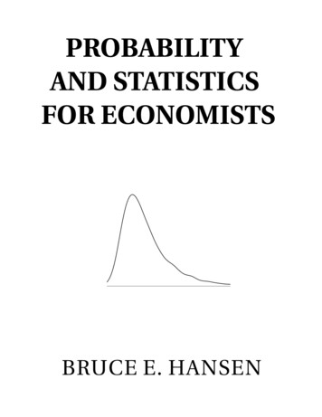
Probability and Mathematical Statistics353Next, we compute the variance of the population X. The variance of X isgiven by V ar(X) E X 2 E(X)2 2 113 6x (1 x) dx 20 11 6x3 (1 x) dx 40 1 6 B(4, 2) 4 Γ(4) Γ(2)1 6 Γ(6)4 11 6 20465 20 201 .20Since X1 and X2 have the same distribution as the population X, we getV ar(X1 ) 1 V ar(X2 ).20Hence, the variance of the sample sum Y is given byV ar(Y ) V ar (X1 X2 ) V ar (X1 ) V ar (X2 ) 2 Cov (X1 , X2 ) V ar (X1 ) V ar (X2 )11 20 201 .10Example 13.2. Let X1 and X2 be a random sample of size 2 from a distribution with density 1f (x) 4for x 1, 2, 3, 40otherwise.What is the distribution of the sample sum Y X1 X2 ?

Sequences of Random Variables and Order Statistics354Answer: Since the range space of X1 as well as X2 is {1, 2, 3, 4}, the rangespace of Y X1 X2 isRY {2, 3, 4, 5, 6, 7, 8}.Let g(y) be the density function of Y . We want to find this density function.First, we find g(2), g(3) and so on.g(2) P (Y 2) P (X1 X2 2) P (X1 1 and X2 1) P (X1 1) P (X2 1)(by independence of X1 and X2 ) f (1) f (1) 111 .4416g(3) P (Y 3) P (X1 X2 3) P (X1 1 and X2 2) P (X1 2 and X2 1) P (X1 1) P (X2 2) P (X1 2) P (X2 1) f (1) f (2) f (2) f (1) 11112 .444416(by independence of X1 and X2 )

Probability and Mathematical Statistics355g(4) P (Y 4) P (X1 X2 4) P (X1 1 and X2 3) P (X1 3 and X2 1) P (X1 2 and X2 2) P (X1 3) P (X2 1) P (X1 1) P (X2 3) P (X1 2) P (X2 2)(by independence of X1 and X2 ) f (1) f (3) f (3) f (1) f (2) f (2) 111111 4444443 .16Similarly, we getg(5) 4,16g(6) 3,16g(7) 2,16g(8) 1.16Thus, putting these into one expression, we getg(y) P (Y y) y 1 f (k) f (y k)k 1 4 y 5 ,16Remark 13.1. Note that g(y) y 1 y 2, 3, 4, ., 8.f (k) f (y k) is the discrete convolutionk 1of f with itself. The concept of convolution was introduced in chapter 10.The above example can also be done using the moment generating func-

Sequences of Random Variables and Order Statistics356tion method as follows:MY (t) MX1 X2 (t) MX1 (t) MX2 (t) t t e e2t e3t e4te e2t e3t e4t 44 t 2t3t4t 2e e e e 4e2t 2e3t 3e4t 4e5t 3e6t 2e7t e8t .16Hence, the density of Y is given byg(y) 4 y 5 ,16y 2, 3, 4, ., 8.Theorem 13.1. If X1 , X2 , ., Xn are mutually independent random variables with densities f1 (x1 ), f2 (x2 ), ., fn (xn ) and E[ui (Xi )], i 1, 2, ., nexist, then n n11Eui (Xi ) E[ui (Xi )],i 1i 1where ui (i 1, 2, ., n) are arbitrary functions.Proof: We prove the theorem assuming that the random variablesX1 , X2 , ., Xn are continuous. If the random variables are not continuous,then the proof follows exactly in the same manner if one replaces the integralsby summations. SinceEn1ui (Xi )i 1 E(u1 (X1 ) · · · un (Xn )) ···u1 (x1 ) · · · un (xn )f (x1 , ., xn )dx1 · · · dxn ···u1 (x1 ) · · · un (xn )f1 (x1 ) · · · fn (xn )dx1 · · · dxn u1 (x1 )f1 (x1 )dx1 · · ·un (x1 )fn (xn )dxn E (u1 (X1 )) · · · E (un (Xn ))n1 E (ui (Xi )) ,i 1

Probability and Mathematical Statistics357the proof of the theorem is now complete.Example 13.3. Let X and Y be two random variables with the joint density (x y)efor 0 x, y f (x, y) 0otherwise.What is the expected value of the continuous random variable Z X 2 Y 2 XY 2 X 2 X?Answer: Sincef (x, y) e (x y) e x e y f1 (x) f2 (y),the random variables X and Y are mutually independent. Hence, the expected value of X is E(X) x f1 (x) dx 0 xe x dx0 Γ(2) 1.Similarly, the expected value of X 2 is given by E X2 x2 f1 (x) dx0 x2 e x dx0 Γ(3) 2.Since the marginals of X and Y are same, we also get E(Y ) 1 and E(Y 2 ) 2. Further, by Theorem 13.1, we get E [Z] E X 2 Y 2 XY 2 X 2 X E X2 X Y 2 1 E X2 X E Y 2 1(by Theorem 13.1) 2 2 E X E [X] E Y 1 (2 1) (2 1) 9.

Sequences of Random Variables and Order Statistics358Theorem 13.2. If X1 , X2 , ., Xn are mutually independent random variables with respective means µ1 , µ2 , ., µn and variances σ12 , σ22 , ., σn2 , then nthe mean and variance of Y i 1 ai Xi , where a1 , a2 , ., an are real constants, are given byµY n ai µiσY2 andi 1n a2i σi2 .i 1Proof: First we show that µY ni 1ai µi . SinceµY E(Y ) En ai Xii 1 n i 1n ai E(Xi )ai µii 1we have asserted result. Next we show σY2 ni 1a2i σi2 . ConsiderσY2 V ar(Y ) V ar (ai Xi )n a2i V ar (Xi )i 1 n a2i σi2 .i 1This completes the proof of the theorem.Example 13.4. Let the independent random variables X1 and X2 havemeans µ1 4 and µ2 3, respectively and variances σ12 4 and σ22 9.What are the mean and variance of Y 3X1 2X2 ?Answer: The mean of Y isµY 3µ1 2µ2 3( 4) 2(3) 18.

Probability and Mathematical Statistics359Similarly, the variance of Y isσY2 (3)2 σ12 ( 2)2 σ22 9 σ12 4 σ22 9(4) 4(9) 72.Example 13.5. Let X1 , X2 , ., X50 be a random sample of size 50 from adistribution with density 1 xθfor 0 x θ ef (x) 0otherwise.What are the mean and variance of the sample mean X?Answer: Since the distribution of the population X is exponential, the meanand variance of X are given byµX θ,and2σX θ2 .Thus, the mean of the sample mean is X1 X2 · · · X50E X E50 501 E (Xi )50 i 1 501 θ50 i 1150 θ θ.50The variance of the sample mean is given by 50 1V ar X V arXi50i 1 250 12 σXi50i 1 250 1 θ250i 1 21 50θ250θ2 .50

Sequences of Random Variables and Order Statistics360Theorem 13.3. If X1 , X2 , ., Xn are independent random variables withrespective moment generating functions MXi (t), i 1, 2, ., n, then the mo nment generating function of Y i 1 ai Xi is given byMY (t) n1MXi (ai t) .i 1Proof: SinceMY (t) M ni 1 n1i 1n1ai Xi (t)Mai Xi (t)MXi (ai t)i 1we have the asserted result and the proof of the theorem is now complete.Example 13.6. Let X1 , X2 , ., X10 be the observations from a randomsample of size 10 from a distribution with density1 21f (x) e 2 x ,2π x .What is the moment generating function of the sample mean?Answer: The density of the population X is a standard normal. Hence, themoment generating function of each Xi is1 2MXi (t) e 2 t ,i 1, 2, ., 10.The moment generating function of the sample mean isMX (t) M 101Xii 1 10 101 MXii 1 101(t)1t10 t2e 200i 1 1" t2 #10 e 200 e 10 Hence X N 0,110 .t22 .

Probability and Mathematical Statistics361The last example tells us that if we take a sample of any size from anormal population, then the sample mean also has a normal distribution.The following theorem says that a linear combination of random variableswith normal distributions is again normal.Theorem 13.4. If X1 , X2 , ., Xn are mutually independent random variables such that Xi N µi , σi2 ,i 1, 2, ., n.n Then the random variable Y ai Xi is a normal random variable withi 1meanµY nn i 1ai µiσY2 andn a2i σi2 ,i 1 2 2i 1 ai σi . Proof: Since each Xi N µi , σi2 , the moment generating function of eachXi is given by1 2 2MXi (t) eµi t 2 σi t .that is Y Ni 1 ai µi , nHence using Theorem 13.3, we haven1MY (t) MXi (ai t) i 1n112 2eµi t 2 σi ti 1 n 2 2 n1 e i 1 µi t 2 i 1 σi t .Thus the random variable Y Nn ai µi ,i 1n a2i σi2 . The proof of thei 1theorem is now complete.Example 13.7. Let X1 , X2 , ., Xn be the observations from a random sample of size n from a normal distribution with mean µ and variance σ 2 0.What are the mean and variance of the sample mean X?Answer: The expected value (or mean) of the sample mean is given byn 1 E X E (Xi )n i 1 n1 µn i 1 µ.

Sequences of Random Variables and Order Statistics362Similarly, the variance of the sample mean isn V ar X V ar i 1Xin n 2 1i 1nσ2 σ2.nThis example along with the previous theorem says that if we take a randomsample of size n from a normal population with mean µ and variance σ 2 ,2then the sample mean is also normal with mean µ and variance σn , that isX N µ,σ2n.Example 13.8. Let X1 , X2 , ., X64 be a random sample of size 64 from anormal distribution with µ 50 and σ 2 16. What are P (49 X8 51) and P 49 X 51 ?Answer: Since X8 N (50, 16), we getP (49 X8 51) P (49 50 X8 50 51 50) 49 50X8 5051 50 P 444 1X8 501 P 444 11 P Z 44 1 2P Z 14 0.1974(from normal table). By the previous theorem, we see that X N 50,1664 . Hence P 49 X 51 P 49 50 X 50 51 50 49 50X 5051 50 P 16641664 1664X 50 P 2 2 1664 P ( 2 Z 2) 2P (Z 2) 1 0.9544(from normal table).

Probability and Mathematical Statistics363This example tells us that X has a greater probability of falling in an intervalcontaining µ, than a single observation, say X8 (or in general any Xi ).Theorem 13.5. Let the distributions of the random variables X1 , X2 , ., Xnbe χ2 (r1 ), χ2 (r2 ), ., χ2 (rn ), respectively. If X1 , X2 , ., Xn are mutually in ndependent, then Y X1 X2 · · · Xn χ2 ( i 1 ri ).Proof: Since each Xi χ2 (ri ), the moment generating function of each Xiis given byriMXi (t) (1 2t) 2 .By Theorem 13.3, we haveMY (t) n1i 1MXi (t) n1ri(1 2t) 2 (1 2t) 21 ni 1ri.i 1 nHence Y χ2 ( i 1 ri ) and the proof of the theorem is now complete.The proof of the following theorem is an easy consequence of Theorem13.5 and we leave the proof to the reader.Theorem 13.6. If Z1 , Z2 , ., Zn are mutually independent and each oneis standard normal, then Z12 Z22 · · · Zn2 χ2 (n), that is the sum ischi-square with n degrees of freedom.The following theorem is very useful in mathematical statistics and itsproof is beyond the scope of this introductory book.Theorem 13.7. If X1 , X2 , ., Xn are observations of a random sample of size n from the normal distribution N µ, σ 2 , then the sample mean X n n1122i 1 Xi and the sample variance S n 1i 1 (Xi X) have thenfollowing properties:(A) X and S 2 are independent, and2(B) (n 1) Sσ2 χ2 (n 1).Remark 13.2. At first sight the statement (A) might seem odd since thesample mean X occurs explicitly in the definition of the sample varianceS 2 . This remarkable independence of X and S 2 is a unique property thatdistinguishes normal distribution from all other probability distributions.Example 13.9. Let X1 , X2 , ., Xn denote a random sample from a normaldistribution with variance σ 2 0. If the first percentile of the statistics2 nW i 1 (Xiσ X)is 1.24, where X denotes the sample mean, what is the2sample size n?

Sequences of Random Variables and Order StatisticsAnswer:3641 P (W 1.24)100n (Xi X)2 P 1.24σ2i 1 S2 P (n 1) 2 1.24σ 2 P χ (n 1) 1.24 .Thus from χ2 -table, we getn 1 7and hence the sample size n is 8.Example 13.10. Let X1 , X2 , ., X4 be a random sample from a normal distribution with unknown mean and variance equal to 9. Let S 2 2 4 1i 1 Xi X . If P S k 0.05, then what is k?3Answer: 0.05 P S 2 k 2 3S3 P k99 3 P χ2 (3) k .9From χ2 -table with 3 degrees of freedom, we get3k 0.359and thus the constant k is given byk 3(0.35) 1.05.13.2. Laws of Large NumbersIn this section, we mainly examine the weak law of large numbers. Theweak law of large numbers states that if X1 , X2 , ., Xn is a random sampleof size n from a population X with mean µ, then the sample mean X rarelydeviates from the population mean µ when the sample size n is very large. Inother words, the sample mean X converges in probability to the populationmean µ. We begin this section with a result known as Markov inequalitywhich is need to establish the weak law of large numbers.

Probability and Mathematical Statistics365Theorem 13.8 (Markov Inequality). Suppose X is a nonnegative randomvariable with mean E(X). ThenE(X)tP (X t) for all t 0.Proof: We assume the random variable X is continuous. If X is not continuous, then a proof can be obtained for this case by replacing the integralswith summations in the following proof. Since E(X) xf (x)dx t xf (x)dx xf (x)dxtxf (x)dx t tf (x)dxt tbecause x [t, ) f (x)dxt t P (X t),we see thatP (X t) E(X).tThis completes the proof of the theorem.In Theorem 4.4 of the chapter 4, Chebychev inequality was treated. LetX be a random variable with mean µ and standard deviation σ. Then Chebychev inequality says thatP ( X µ kσ) 1 1k2for any nonzero positive constant k. This result can be obtained easily usingTheorem 13.8 as follows. By Markov inequality, we haveP ((X µ)2 t2 ) E((X µ)2 )t2for all t 0. Since the events (X µ)2 t2 and X µ t are same, wegetE((X µ)2 )P ((X µ)2 t2 ) P ( X µ t) t2

Sequences of Random Variables and Order Statistics366for all t 0. Henceσ2.t2in the above equality, we see thatP ( X µ t) Letting k σt1.k2P ( X µ kσ) Hence1.k2The last inequality yields the Chebychev inequality1 P ( X µ kσ) P ( X µ kσ) 1 1.k2Now we are ready to treat the weak law of large numbers.Theorem 13.9. Let X1 , X2 , . be a sequence of independent and identicallydistributed random variables with µ E(Xi ) and σ 2 V ar(Xi ) fori 1, 2, ., . Thenlim P ( S n µ ε) 0n for every ε. Here S n denotesX1 X2 ··· Xn.nProof: By Theorem 13.2 (or Example 13.7) we haveE(S n ) µandV ar(S n ) σ2.nBy Chebychev’s inequalityP ( S n E(S n ) ε) V ar(S n )ε2for ε 0. Henceσ2.n ε2Taking the limit as n tends to infinity, we getP ( S n µ ε) σ2n n ε2lim P ( S n µ ε) limn which yieldslim P ( S n µ ε) 0n and the proof of the theorem is now complete.

Probability and Mathematical Statistics367It is possible to prove the weak law of large numbers assuming only E(X)to exist and finite but the proof is more involved.The weak law of large numbers says that the sequence of sample means3 S n n 1 from a population X stays close to population mean E(X) mostof the times. Let us consider an experiment that consists of tossing a coininfinitely many times. Let Xi be 1 if the ith toss results in a Head, and 0otherwise. The weak law of large numbers says that2Sn 1X1 X2 · · · Xn n2asn (13.0)but it is easy to come up with sequences of tosses for which (13.0) is false:H H H H H H H H H H H HH H T H H T H H T H H T··· ······ ···The strong law of large numbers (Theorem 13.11) states that the set of “badsequences” like the ones given above has probability zero.Note that the assertion of Theorem 13.9 for any ε 0 can also be writtenaslim P ( S n µ ε) 1.n The type of convergence we saw in the weak law of large numbers is notthe type of convergence discussed in calculus. This type of convergence iscalled convergence in probability and defined as follows.Definition 13.1. Suppose X1 , X2 , . is a sequence of random variables defined on a sample space S. The sequence converges in probability to therandom variable X if, for any ε 0,lim P ( Xn X ε) 1.n In view of the above definition, the weak law of large numbers states thatthe sample mean X converges in probability to the population mean µ.The following theorem is known as the Bernoulli law of large numbersand is a special case of the weak law of large numbers.Theorem 13.10. Let X1 , X2 , . be a sequence of independent and identicallydistributed Bernoulli random variables with probability of success p. Then,for any ε 0,lim P ( S n p ε) 1n

Sequences of Random Variables and Order Statisticswhere S n denotes368X1 X2 ··· Xn.nThe fact that the relative frequency of occurrence of an event E is verylikely to be close to its probability P (E) for large n can be derived fromthe weak law of large numbers. Consider a repeatable random experimentrepeated large number of time independently. Let Xi 1 if E occurs on theith repetition and Xi 0 if E does not occur on ith repetition. Thenµ E(Xi ) 1 · P (E) 0 · P (E) P (E)for i 1, 2, 3, .andX1 X2 · · · Xn n N (E)where N (E) denotes the number of times E occurs. Hence by the weak lawof large numbers, we have N (E)X1 X2 · · · Xnlim P P (E) ε lim P µ εn n nn lim P S n µ εn 0.Hence, for large n, the relative frequency of occurrence of the event E is verylikely to be close to its probability P (E).Now we present the strong law of large numbers without a proof.Theorem 13.11. Let X1 , X2 , . be a sequence of independent and identicallydistributed random variables with µ E(Xi ) and σ 2 V ar(Xi ) fori 1, 2, ., . Thenlim P ( S n µ) ε) 0n for every ε. Here S n denotesX1 X2 ··· Xn.nThe type convergence in Theorem 13.11 is called almost sure convergence.The notion of almost sure convergence is defined as follows.Definition 13.2 Suppose the random variable X and the sequenceX1 , X2 , ., of random variables are defined on a sample space S. The sequence Xn (w) converges almost surely to X(w) if 4Pw S lim Xn (w) X(w) 1.n It can be shown that the convergence in probability implies the almostsure convergence but not the converse.

Probability and Mathematical Statistics36913.3. The Central Limit TheoremnConsider a random sample of measurement {Xi }i 1 . The Xi ’s are identically distributed and their common distribution is the distribution of thepopulation. We have seen that if the population distribution is normal, thenthe sample mean X is also normal. More precisely, if X1 , X2 , ., Xn is arandom sample from a normal distribution with densityf (x) 1 x µ 21 e 2 ( σ )σ 2π thenX Nµ,σ2n .The central limit theorem (also known as Lindeberg-Levy Theorem) statesthat even though the population distribution may be far from being normal,still for large sample size n, the distribution of the standardized sample meanis approximately standard normal with better approximations obtained withthe larger sample size. Mathematically this can be stated as follows.Theorem 13.12 (Central Limit Theorem). Let X1 , X2 , ., Xn be a random sample of size n from a distribution with mean µ and variance σ 2 ,then the limiting distribution ofZn X µ σnis standard normal, that is Zn converges in dist

In this book we present an introduction to probability and mathematical statistics and it is intended for students already having some elementary mathematical background. It is intended for a one-year senior level undergraduate and beginning graduate level course in probability theory and ma