Transcription
Approximating the Distribution for Sumsof Products of Normal VariablesRobert Ware1 and Frank Lad2AbstractWe consider how to calculate the probability that the sum of the productof variables assessed with a Normal distribution is negative. The analysis ismotivated by a specific problem in electrical engineering. To resolve the problem, two distinct steps are required. First, we consider ways in which we canassess the distribution for the product of two Normally distributed variables.Three different methods are compared: a numerical methods approximation,which involves implementing a numerical integration procedure on MATLAB,a Monte Carlo construction and an approximation to the analytic result usingthe Normal distribution. The second step considers how to assess the distribution for the sum of the products of two Normally distributed variablesby applying the Convolution Formula. Finally, the two steps are combinedto compute the distribution for the sum of products of Normally distributedvariables, and thus to calculate the probability that this sum of productsis negative. The problem is also approached directly, using a Monte Carloapproximation.Key Words: Product of Normal variables; Numerical integration;Differential continuous phase frequency shift keying; Convolutions;Moment generating function.1IntroductionThe work discussed in this Report originated from a problem posed by Griffin (2000)who was interested in calculating the probability that the sum of the product of variables assessed with a Normal distribution was negative. Previous work involving thedistribution of the product of two Normally distributed variables has been undertaken by Craig (1936), who was the first to determine the algebraic form of themoment-generating function of the product. Aroian et al. (1978) proved that, undercertain conditions, the product of two Normally distributed variables approachesthe standardised Pearson type III distribution. Cornwell et al. (1978) described thenumerical evaluation of the product. Conradie and Gupta (1987) presented basic12Research Fellow, School of Population Health, The University of QueenslandResearch Associate, Department of Mathematics and Statistics, University of Canterbury1
distributional results of the quadratic forms of p-variate complex Normal distributions. Their results were developed in terms of characteristic functions. However,these results were found to be too theoretical to be easily transferred to a problemas applied as the one under investigation.While the work of Craig (1936) is relatively old, it is not at all well-knownamong statisticians. Indeed we did not even learn of it until we had rediscovered itourselves in developing this Thesis. At that time we also learned of the researchesof Aroian et al. (1978) and Cornwell et al. (1978). Nonetheless, recent advances incomputing power and graphics have allowed us to make several useful advances onthe consulting problem that had been posed.To calculate the probability that the sum of products of variables assessed ashaving a Normal distribution is negative, two distinct steps are required. The firststep considers ways in which we can assess the distribution for the product of twoNormally distributed variables. The second step involves identifying the distributionwhen summing a number of these products together.In Section 2, the process of differential continuous phase frequency shift keying isbriefly introduced as it was studied by Griffin (2000). The relevance of the distribution of sums of products of Normally distributed variables is recognised. In Section 3we assess the distribution for Y X1 X2 , the product of two independent Normallydistributed variables. We compare three different methods: a numerical methodsapproximation, which involves implementing a numerical integration procedure onMATLAB, a Monte Carlo construction and an approximation to the analytic resultusing the Normal distribution. The numerical integration procedure involves thejoint distribution of Y and X2 . We discover that f (y, x2 ) has a simple singularityat (0, 0), and discuss the resulting consequences for the numerical integration. Thenumerical integration is implemented via MATLAB and Maple subroutines, eliminating the need for evaluation via statistical tables. New graphics are presentedto aid understanding of the shape of the distribution Y . We undertake a specificanalysis of the skewness of the product of two Normally distributed variables whenthe multiplicands are correlated. Section 4 considers how to assess the distributionfor the sum of the products of two Normally distributed variables by applying theConvolution Formula. This technique is demonstrated using the products previously2
obtained via numerical integration. A computational procedure for approximatingthe required distribution using convolutions is developed. In Section 5 the methods of Sections 3 and 4 are combined to compute the distribution for the sum ofproducts of Normally distributed variables, and thus to calculate the probabilitythat this sum of products is negative. We also approach this problem directly, usinga Monte Carlo approximation. Finally, in Section 6 a summary of the Report ispresented.2Introduction to Differential Continuous PhaseFrequency Shift KeyingDifferential continuous phase frequency shift keying is a procedure for transmittingand decoding a signal that has been intentionally disturbed by noise. Interest centreson how accurately the receiver can decode the original signal.In a typical encoding problem the original signal, called s(t), is differentiallyencoded and then transmitted. During transmission over a channel, Gaussian noise,w(t), is added to the signal so that the received signal, y(t), is a combination of thetransmitted signal and noise, i.e. y(t) s(t) w(t). The ratio of s(t) to the standarddeviation of w(t) is called the “signal to noise ratio”. The estimate of the originalsignal is called the hypothesised signal, and is denoted ŝ(t). The receiver uses adecoder to minimise the squared Euclidean distance between the transmitted signaland the hypothesised signal. The performance of the receiver can be characterisedby the probability of error between s(t) and ŝ(t). As is common in problems ofelectrical engineering, the problem is expressed via complex valued functions andthe practical solution is determined by the real component of the complex solution.In the problem posed by Griffin (2000), interest centres on the probability that thereal component of the error metric between the transmitted and hypothesised signalsis less than 0, that is, P [Re(Me (s, ŝ)) 0].The transmitted signal consists of a finite number of received signals, say N of3
them, so that y ξ 1 y ξ 2 . . y yt . . y ξ N s ξ 1 s ξ 2 st w ξ 1 w ξ 2 . . wt.s ξ N w ξ N s w (1)where ξ is a positive integer. In the case of the problem posed, the error metric isachieved as the real component of a complex expression and is representable asMe (s, ŝ) 2NξXt 1(yR,t yR,t ξ bR,t yR,t yI,t ξ bI,t yI,t yR,t ξ bI,t yI,t yI,t ξ bR,t ) .(2)The coefficients bR,t and bI,t are real constants, predetermined along with the meansof yR,t and yI,t by the signal that is sent. Furthermore the added noise is constructedso that yR,t yI,t 20 µR,t σw 0 20 µI,t 0 σw , N 2 µ 0 σw R,t ξ 0 y R,t ξ yI,t ξ µI,t ξ 000 0 0 . 0 2σw2are determined by the signal toThe relative size of the different values of µ and σwnoise ratio. For problems of this type it is usual practise to set all values of µ equal2to 1, and then set σwto achieve the required signal to noise ratio for the problemunder investigation. N is usually given the value 2 or 3, ξ is set to be some value of2k , where k 0, and bR,t and bI,t are both set to 1.Our interest centres on finding the probability that the real component of theerror metric is negative. In Sections 3 and 4 our focus will be on the shape of thedistribution of the error metric. Thus, we shall disregard the coefficient “2” fromEquation 2.Essentially, the problem posed by P [Re (Me (s, ŝ)) 0] requires that we be ableto compute probabilities for the sum of products of Normal variables. We now turnto a study of this problem in a general context.4
3The Simplest Problem of the Product of TwoNormal VariablesThe form of the simplest problem we consider is a bivariate Normal distributionwith independent variables: µ1 X1 , N X2µ2σ120The joint density of X1 and X2 is 11f (x1 , x2 ) e 22πσ1 σ2³x1 µ1σ1 2 21³x2 µ2σ2 0 .σ22 2for all x1 , x2 R(3)Our interest centres on the distribution of the product X1 X2 . To simplify notation,for the remainder of this Report we let Y X1 X2 .3.1A Numerical Methods ApproximationThe conditional distribution of Y (X2 x2 ), and the distribution of X2 , are:Y X2 x2 N (x2 µ1 , x22 σ12 ), N (µ2 , σ22 ).X2Thus we can find the joint density of X2 and Y :f (y, x2 ) f (y x2 )f (x2 ) 12 (x2 µ2 )2 21 2 (y x2 µ1 )211 e 2σ2e 2x2 σ12π x2 σ12πσ2 121e 2σ1 2π x2 σ1 σ2³y µ1x2 2 1(x2 µ2 )22σ 22.(4)To find the marginal density f (y), we need to integrate f (y x2 )f (x2 ) withrespect to x2 . In other words we solvef (y) Z Z f (y x2 )f (x2 )dx2f (y, x2 )dx2 .(5) This integration can be undertaken using the numerical integration procedure on themathematical computer package MATLAB called “quad8”, which works by using5
an adaptive recursive Newton Cotes 8 panel rule. A numeric value ofRf (y, x2 )dx2is obtained for an array of points in the domain of Y . These points are all extremelyclose to one another and essentially cover all realistic possibilities for y. We consider the density as essentially uniform on these tight intervals. These integratedvalues are then summed and normalised. The same numerical integration can beperformed on the computer package Maple. The calling sequence “evalf(Int)” invokes a Clenshaw-Curtis quadrature method. As in MATLAB, a numeric value ofRf (y, x2 )dx2 is obtained for an array of points in the domain of Y . We shall comparethe results of these two integration procedures.3.1.1Case 1: µ1 1, µ2 0.5, σ 2 1, cov(X1 , X2 ) 0.Consider the case X1 1 1 0 N , .X20.50 1The joint density of X1 and X2 is called a circular Normal density, and by Equation 3f (x1 , x2 ) 1 21 (x21 2x1 x22 x2 45 )e.2π(6)We can view f (x1 , x2 ) in three dimensions, Figure 1, as well as by continuous contours in two dimensions, Figure 2. Figure 1 shows that f (x1 , x2 ) is a bivariateNormal surface with a maximum at (1, 0.5). In Figure 2 the contours of constantprobability density for f (x1 , x2 ) are drawn at 0.005, 0.055, 0.105 and 0.155. Theisoproduct lines are shown for x1 x2 1, 2, 3, 4, 5.The joint density f (y, x2 ) can be easily calculated. By Equation 4 we have 121ef (y, x2 ) 2π x2 ³y2 x2y x22 x2 54x222 .(7)A study of f (y, x2 ) shows us that:1. The domain for (X2 , Y ) is R2 {(0, y) y 6 0}, because y x1 x2 and ifx2 0, y must be 0.2. When x2 and y are both large, f (y, x2 ) 0.3. At pairs (y, x2 ) 6 (0, 0) the density will be what it is — varying real values.6
0.160.14f (x1 , x2 )0.120.10.080.060.040.020420 2 3x2 210 1234x1Figure 1: Joint density of X1 N (1, 1) and X2 N (0.5, 1) displayed inthree dimensions.5432x210 1 2 3 4 5 5 4 3 2 10x112345Figure 2: Constant density contours for the joint density f (x1 , x2 ) displayed in two dimensions, along with the isoproduct lines for X1 X2 .7
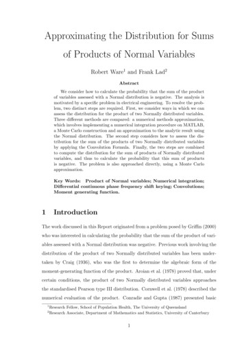
3000f (y, x2 .000102e–054e–056e–058e–050.0001x2Figure 3: The joint density f (y, x2 ) displayed in three dimensions forCase 1. For clarity the density is only displayed for f (y, x2 ) 3000.4. The joint density has a simple singularity at (y, x2 ) (0, 0). The directionfrom which the domain point (y, x2 ) (c, 0) is approached does not affect thefact that limx2 0 f (y, x2 ) does not exist. To see this, let y kx2 for some realk. Then Equation 7 becomesf (y, x2 ) 51122e 2 (k 2k x2 x2 4 ) .2π x2 (8)In this form it is easy to see that f (y, x2 ) as x2 0 for every real k.Moreover, it is evident directly from Equation 8 that for any fixed value ofy 6 0, limx2 0 f (y, x2 ) 0. (Remember that points (y, x2 ) (y, 0) for y 6 0are missing from the domain of (Y, X2 ).)Let us now examine the density f (y, x2 ) as produced by Maple in Figure 3 andMATLAB in Figure 4. Figure 3 displays a standard three dimensional picture ofthe function, while Figure 4 shows the isodensity contours. The larger contourscorrespond to low density values, the smaller contours correspond to high densityvalues.8
(b)0.020.150.0150.10.010.050.005yy(a)0.200 0.05 0.005 0.1 0.01 0.15 0.015 0.2 0.2 0.10x20.1 0.02 0.020.2 0.010x20.010.02Figure 4: Contours for the joint density f (y, x2 ) displayed in two dimensions for Case 1. In (a) contours are plotted at f (y, x2 ) 1, 2, 3, 4, 5. In (b)contours are plotted at f (y, x2 ) 10, 20, 30, 40, 50.A consequence of f (y, x2 ) being undefined when x2 0 and y 6 0 is that tointegrate f (y, x2 ) numerically we need to separate the integral into two domains forX2 : x2 ( , 0) and x2 (0, ). Once the positive and negative halves havebeen integrated individually, they are added together and normalised to give themarginal density f (y). In MATLAB it took 10 minutes to complete this numericalintegration using interval widths of 0.01. Figure 5 demonstrates that the marginaldensity is neither Normal or symmetric. Notice there is a slight fluctuation in f (y)at y 2.3. Similar, and far more marked, fluctuations occur in Case 2, and arediscussed in the next subsection.The density has an asymptote at y 0, but of course we cannot display itgraphically
To calculate the probability that the sum of products of variables assessed as having a Normal distribution is negative, two distinct steps are required. The first step considers ways in which we can assess the distribution for the product of two Normally distributed variables. The second step involves identifying the distribution