Transcription
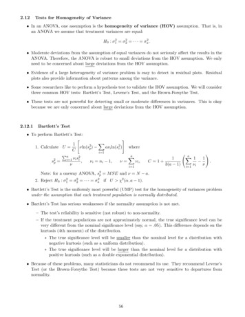
2.12Tests for Homogeneity of Variance In an ANOVA, one assumption is the homogeneity of variance (HOV) assumption. That is, inan ANOVA we assume that treatment variances are equal:H0 : σ12 σ22 · · · σa2 . Moderate deviations from the assumption of equal variances do not seriously affect the results in theANOVA. Therefore, the ANOVA is robust to small deviations from the HOV assumption. We onlyneed to be concerned about large deviations from the HOV assumption. Evidence of a large heterogeneity of variance problem is easy to detect in residual plots. Residualplots also provide information about patterns among the variance. Some researchers like to perform a hypothesis test to validate the HOV assumption. We will considerthree common HOV tests: Bartlett’s Test, Levene’s Test, and the Brown-Forsythe Test. These tests are not powerful for detecting small or moderate differences in variances. This is okaybecause we are only concerned about large deviations from the HOV assumption.2.12.1Bartlett’s Test To perform Bartlett’s Test:"#X11. Calculate U νln(s2p ) aνi ln(s2i ) whereCi 1Paa2Xνi sνi ni 1,ν νi ,s2p i 1 i ,νi 11C 1 3(a 1)aX11 νi ν!.i 1Note: for a oneway ANOVA, s2p M SE and ν N a.2. Reject H0 : σ12 σ22 · · · σa2 if U χ2 (α, a 1). Bartlett’s Test is the uniformly most powerful (UMP) test for the homogeneity of variances problemunder the assumption that each treatment population is normally distributed. Bartlett’s Test has serious weaknesses if the normality assumption is not met.– The test’s reliability is sensitive (not robust) to non-normality.– If the treatment populations are not approximately normal, the true significance level can bevery different from the nominal significance level (say, α .05). This difference depends on thekurtosis (4th moment) of the distribution. The true significance level will be smaller than the nominal level for a distribution withnegative kurtosis (such as a uniform distribution). The true significance level will be larger than the nominal level for a distribution withpositive kurtosis (such as a double exponential distribution). Because of these problems, many statisticians do not recommend its use. They recommend Levene’sTest (or the Brown-Forsythe Test) because these tests are not very sensitive to departures fromnormality.56
2.12.2Levene’s Test To perform Levene’s Test:1. Calculate each zij yij y i· .2. Run an ANOVA on the set of zij values.3. If p-value α, reject Ho and conclude the variances are not all equal. Levene’s Test is robust because the true significance level is very close to the nominal significancelevel for a large variety of distributions. It is not sensitive to symmetric heavy-tailed distributions (such as the double exponential and student’s t distributions).2.12.3Brown-Forsythe Test To perform the Brown-Forsythe Test:1. Calculate each zij yij yei where yei is the median for the ith treatment.2. Run an ANOVA on the set of zij ’s.3. If p-value α, reject Ho and conclude the variances are not all equal. The Brown-Forsythe Test is relatively insensitive to departures from normality. It is not sensitive to skewed distributions (e.g., χ2 ) and extremely heavy-tailed distributions (e.g.,Cauchy). In these cases, it is more robust than Levene’s Test.2.12.4Example of Bartlett’s, Levene’s, and Brown-Forsythe TestsA textile company has five looms that weave cloth. The company is concerned that there may be significantvariability in the strengths of the cloth produces by the looms. Five random samples of cloth are takenfrom the cloth produced by each loom. Each sample is tested and the strength is recorded. The data 613.913.814.0The SAS SystemSAS Output for HOV TestsThe GLM ProcedureclothLevel ofloomNMeanStd Dev15 14.08000000.0836660025 13.92000000.0836660035 14.06000000.1140175445 13.80000000.1581138855 13.82000000.1483239757
The SAS SystemThe GLM ProcedureDependent Variable: clothSourceDFSum ofSquares Mean Square F Value Pr FModel4 0.341600000.08540000Error20 0.296000000.01480000Corrected Total24 0.637600005.770.0030R-Square Coeff Var Root MSE cloth Mean0.5357590.8729570.12165513.93600Source DF Type III SS Mean Square F Value Pr e GLM ProcedureBartlett's Test for Homogeneity ofcloth VarianceSource DF Chi-Square Pr ChiSqloom The 4SAS System2.56890.6323The GLM ProcedureLevene's Test for Homogeneity of cloth VarianceANOVA of Absolute Deviations from Group MeansSum ofDF SquaresSourceloom4Error0.0122MeanSquareF ValuePr F0.003040.670.6179200.09020.00451The SASSystemThe GLM ProcedureBrown and Forsythe's Test for Homogeneity of cloth VarianceANOVA of Absolute Deviations from Group MediansDFSum ofSquaresMeanSquareF ValuePr ource From the following analysis in SAS, the p-values for Bartlett’s Test, Levene’s Test, and the BrownForsythe are .6323, .6179, and .6897, respectively. Therefore, we would fail to reject H0 : σ12 σ22 σ32 σ42 σ52 . Therefore, the HOV assumptionsis reasonably met for the oneway ANOVA. And, assuming there are no serious violations of any other assumptions, we would rejectH0 :for the oneway ANOVA.58
SAS Code for HOV TestsDM ’LOG; CLEAR; OUT; CLEAR;’;ODS GRAPHICS ON;ODS PRINTER PDF file ’C:\COURSES\ST541\HOVTEST.PDF’;OPTIONS NODATE *********;*** 5 Looms,Response Cloth Output,n 5 ***;*** Bartlett’s, Brown-Forsythe, Levene’s Tests ****;DATA in; INPUT loom cloth @@; CARDS;1 14.0 1 14.1 1 14.2 1 14.0 1 14.12 13.9 2 13.8 2 13.9 2 14.0 2 14.03 14.1 3 14.2 3 14.1 3 14.0 3 13.94 13.6 4 13.8 4 14.0 4 13.9 4 13.75 13.8 5 13.6 5 13.9 5 13.8 5 14.0;PROC GLM DATA in;CLASS loom;MODEL cloth loom / ss3 ;MEANS loom / HOVTEST BARTLETT;MEANS loom / HOVTEST BF;MEANS loom / HOVTEST LEVENE(TYPE ABS);ODS GRAPHICS OFF;RUN;2.12.5Data Analysis Options When the HOV Assumption is Not Valid If we reject H0 : σ12 σ22 · · · σa2 , then what options do we have to analyze the data? We willconsider the following two options:1. Weighted least squares.2. Using a variance stabilizing transformation.59
2.13Weighted Least Squares Linear regression models (such as the models used in this course) that have a non-constant variancestructure (heterogeneity of variance) can be fitted by the weighted least squares (WLS) method. With the WLS method, the squared deviation between the observed data value and the predictedvalue (yi ybi )2 is multiplied by a weight wi . This weight is inversely proportional to the variance ofyi . For simple linear regression, the WLS function is W (β0 , β1 ) To find the least squares normal equations, simultaneously solve W/ β0 0 and W/ β1 0.The WLS normal equations are:nXwi y i βb0i 1nXwi x i y i βb0i 1nXi 1nXwi βb1nXwi x ii 1wi xi βb1i 1nXwi x2ii 1The solution βb0 and βb1 to these equations are the WLS solutions. In some cases, the weights are known. For example, if an observed yi is actually the mean on niobservations and assuming the original observations comprising the mean have constant variance σ 2 ,then the variance of yi is σ 2 /ni making the weights wi ni . For a one factor CRD, the WLS function isW (µ, τ1 , . . . , τa ) To find the least squares normal equations, you simultaneously solve W/ µ 0 and W/ τi 0 for i 1, 2, . . . , a.After algebraic manipulation, this yields the following WLS normal equations: nininiaa Xa XXXXX τbiwij wij yij µbwij i 1 j 1niXj 1i 1 j 1wij yij µbniXwij τbij 1i 1niXj 1wij for i 1, 2, . . . , aj 1The solution to these (a 1) equations subject to one constraint (such assolutions.Pai 1 τi 0) are the WLS However, because the variance σi2 of yij is typically unknown, we need to estimate the weight 1/σi2from the data. For the one-factor CRD, we know the sample variance s2i for treatment i is an unbiased estimate ofσi2 (E(s2i ) σi2 ). The estimated weight is wbij 1/s2i . SAS and Minitab will perform a WLS analysis. You just have to supply the weights.60
2.13.1Weighted Least Squares (WLS) ExampleEXAMPLE: A company wants to test the effectiveness of a new chemical disinfectant. Six dosage levelswere considered (1 through 5 grams per 100 ml). The experiment involved applying equal amounts of thedisinfectant at each level to a surface that was covered with a common bacteria. The results are givenbelow. The design was completely 13161926152327Dose55555555The sample variances s2i ares21 s22 s23 s24 s25 w3 w4 w5 Thus, the weights 1/s2i arew1 w2 SAS Output for WLS ExampleSAMPLE VARIANCES AND WEIGHTS FOR EACH TREATMENT trtObs trtvar ywgt1122 14.2857 0.070003.6429 0.27451WEIGHTED LEAST SQUARES EXAMPLE WITH BONFERRONI MCPTheProcedure3 GLM3 13.83930.07226ependent Variable: yWeight: wgtSourceDFModel44 27.4286 0.0364655 38.1250 0.02623Sum ofSquares Mean Square F Value Pr F4 207.5551273Error35Corrected Total39 242.555127335.000000051.888781811.86288 .00011.0000000R-Square Coeff Var Root MSE0.85570351.891.000000y Mean8.429653Source DF Type III SS Mean Square F Value Pr Ftrt40F51.89Prob F .00014 207.555127351.8887818Distribution of y6151.89 .0001F51.89Prob F .0001%2230273232432926
WEIGHTED LEAST SQUARES EXAMPLE WITH BONFERRONI MCPThe GLM ProcedureBonferroni (Dunn) t Tests for yNote: This test controls the Type I experimentwise error rate, but it generally has a higher Type II error rate than Tukey's for all pairwisecomparisons.Alpha0.05Error Degrees of Freedom35Error Mean Square1Critical Value of t2.99605Comparisons significant at the 0.05 level areindicated by tweenComparisonMeans5-410.62502.048719.2013 ***5-317.00009.364224.6358 ***5-220.125012.456427.7936 ***5-126.875020.029233.7208 ***-10.6250 -19.2013-2.0487 ***4-54-36.3750-0.42974-29.50002.658616.3414 ***4-116.250010.345522.1545 ***3-5-17.0000 -24.6358-9.3642 ***3-4-6.3750 .42978.742614.3040 ***-20.1250 -27.7936 -12.4564 ***2-4-9.5000 -16.34142-3-3.1250-8.74262-16.75002.2649-2.6586 ***2.492611.2351 ***1-5-26.8750 -33.7208 -20.0292 ***1-4-16.2500 -22.1545 -10.3455 ***1-3-9.8750 -14.3040-5.4460 ***1-2-6.7500 -11.2351-2.2649 ***DM ’LOG; CLEAR; OUT; CLEAR;’;ODS GRAPHICS ON;ODS PRINTER PDF file ’C:\COURSES\ST541\WLS.PDF’;OPTIONS NODATE NONUMBER;DATA in; INPUT trt y @@; CARDS;1 51 11 31 51 22 132 132 62 72 113 123 163 93 183 164 174 134 164 194 265 225 305 275 325 32;1 62 43 74 155 43123451141423296212345312132726
PROC SORT DATA in; BY trt;PROC MEANS DATA in noprint; BY trt;VAR y;OUTPUT OUT wset VAR var y; -- Sort the data by treatments. -- Calculate and save sample -- variances in ‘wset’.DATA wset; SET wset;wgt 1/var y;DROP FREQ TYPE ; -- Calculate the weights from -- the sample variance in wset.PROC PRINT DATA wset;TITLE ’SAMPLE VARIANCES AND WEIGHTS FOR EACH TREATMENT trt’;DATA in; MERGE in wset; BY trt; -- Attach the weights by treatment.PROC GLM DATA in;WEIGHT wgt; -- Include the WEIGHT statement.CLASS trt;MODEL y trt / SS3;MEANS trt / BON;TITLE ’WEIGHTED LEAST SQUARES EXAMPLE WITH BONFERRONI MCP’;RUN;2.14Variance Stabilizing Transformations If the homogeneity of variance assumption is only moderately violated, the F -test results are slightlyaffected when the design is balanced (equal ni ’s). No transformation should be considered. If the homogeneity of variance assumption is either (i) seriously violated or (ii) moderately violatedwith very different ni sample sizes (serious imbalance), then the effects on the F -test are more serious.– If the treatments having the larger variances have the smaller sample sizes, the true Type I erroris larger than the nominal level.– If the treatments having the larger variances have the larger sample sizes, the true Type I erroris smaller than the nominal level. A common approach to deal with nonconstant variance (heterogeneity of variance) is to apply avariance-stabilizing transformation of the response that will equalize the variances across treatments. We then perform the ANOVA on the transformed data. Sometimes the variance of the response increases or decreases as the mean of the response increases.If this is the case, the residuals vs predicted values plot would have a funnel shape. This is when avariance stabilizing transformation may be appropriate. The statistical problem is to use the data to determine the form of the required transformation. Let µi be the mean for treatment i. Suppose the standard deviation of yij is proportional to apower of µi . That is, σi θµαi for some α and θ. θ is called the constant of proportionality.Notationally, we write σi µαi . The symbol means “is proportional to”. The goal is to find a transformation y y λ such that y has constant or near constant varianceacross all treatments. , we no longer have a HOV problem when the This implies that after transforming each yij to yij values.ANOVA is run with the yij It can be shown that the variance is constant if λ 1 α. We will discuss how to estimate α or λ.63
2.14.1The Empirical Method If σi θµαi , then log(σi ) log(θ) α log(µi ). A plot of log(σi ) vs log(µi ) is linear with slope equalto α. Thus, a simple way to estimate α would be to1. Calculate si and y i· for treatment i 1, 2, . . . , a.2. Fit a regression linelog(si ) 3. The least squares estimate of the slope αb is the estimate of α. y λ where λ 1 α4. Transform each yij to yijb.ij values.5. Run the ANOVA on the yij Note that if α 0, then σi θ for all i. Thus, the homogeneity of variance assumption is metwithout a transformation.2.14.2The Box-Cox Procedure Another approach is the Box-Cox procedure which will estimate the value of λ corresponding toλ that maximizes the model R2 .the transformation yij To find the Box-Cox transformation,1. For a sequence of λ values, calculate R2 (λ). R2 (λ) is the model R2 value from the ANOVA onthe transformed y (λ) values.2. Select the λ that maximizes R2 (λ) (which is equivalent to maximizing the likelihood function).λ values.3. Run the ANOVA on the yij SAS can find the Box-Cox transformation using the TRANSREG procedure.2.14.3Transformation Example using the Empirical and Box-Cox MethodsEXAMPLE: We will use the same data used in the WLS 61926152327Dose55555555%2230273232432926 We will see that the recommended transformation is a square root (λ .5) transformation. Thefollowing SAS output contains– The empirical method results and the Box-Cox method results.– The analysis of the original data. Note that the variability increases with the treatment levels(from 1 to 5).– The analysis of the transformed (square root) data. Note that the variability is now nearlyconstant across the treatment levels (from 1 to 5).64
ANOVA TO FIND EMPIRICAL SELECTION OF ALPHAThe GLM ProcedureDependent Variable: logstdFit Plot for logstd2.0EMPIRICAL SELECTION OF ALPHA1stdlogstd logmean3.250 1.90863 0.646381.178652 10.000 3.77964 1.329632.302593 13.125 3.72012 1.313762.574524 19.500 5.23723 1.655792.970415 30.125 6.17454 1.820443.405361.5logstdObs mean1.00.51.52.02.53.0logmeanFit95% Confidence Limits95% Prediction LimitsANOVA TO FIND EMPIRICAL SELECTION OF ALPHAThe GLM ProcedureDependent Variable: logstdSourceDFSum ofSquares Mean Square F Value Pr FModel1 0.795993340.79599334Error3 0.015577650.00519255Corrected Total4 0.81157099153.300.0011R-Square Coeff Var Root MSE logstd Mean0.980806Source5.3251090.0720591.353200DF Type III SS Mean Square F Value Pr 300.0011StandardError t Value Pr t 53030195490.0428310612.380.0011653.5
The GLM ProcedureThe GLM ProcedureFind the Box-Cox Transformation using PROC TRANSREGDistribution of yDistribution of sqrtyThe TRANSREG ProcedureBox-Cox Analysis for y61505sqrtyF100504Log Likelihood30-50Selected λ 0.595% CI-100Selected λ 0.595% CI2-150-200-2-11201LambdaTerms with Pr F 0.05 at the Selected Lambda3trt 1 142trt 2trt 35trttrt 434trtyLevel oftrtN2sqrtyMeanStd DevLevel oftrtNMeanStd Dev183.25000001.9086270318 1.724992610.5600005128 10.00000003.7796447328 3.103590920.6482709938 13.12500003.7201190538 3.587462780.5399584948 19.50000005.2372293748 4.381442830.5884203758 30.12500006.1745445258 5.464890640.5450770066
ANOVA -- ORIGINAL DATAThe GLM ProcedureDependent Variable: ySourceSum ofSquares Mean Square F Value Pr FDFModel4 3323.150000Error35Corrected Total39 4004.400000830.787500681.250000 .000119.464286R-Square Coeff Var Root MSE0.82987542.6829.02523y Mean4.41183515.20000Source DF Type III SS Mean Square F Value Pr FANOVA -- ORIGINAL DATAtrt4 3323.150000830.78750042.68 .0001The GLM ProcedureDependent Variable: yFit Diagnostics for redicted Value0300.2020-10010.17520.100.0010203040Predicted 51000.12540-5-130Cook's D5yResidual10-220Predicted 500-1067Observations40Parameters5Error DF35MSE19.464R-Square0.8299Adj R-Square 0.810440
ANOVA -- SQUARE ROOT TRANSFORMATIONThe GLM ProcedureDependent Variable: sqrtySourceSum ofSquares Mean Square F Value Pr FDFModel4 62.6954658015.67386645Error35 11.681309390.33375170Corrected Total39 74.3767752046.96 .0001R-Square Coeff Var Root MSE sqrty Mean0.84294415.817010.5777123.652476Source DF Type III SS Mean Square F Value Pr FANOVA -- SQUARE ROOT TRANSFORMATIONtrt4 62.6954658015.6738664546.96 .0001The GLM ProcedureDependent Variable: sqrty220.5110.0RStudent1.0RStudentResidualFit Diagnostics for 56Predicted ValueQuantileFit–Mean3025220101000.125Cook's D6550.121.0154Predicted ValuesqrtyResidualPredicted vations40Parameters5Error DF35MSE0.3338R-Square0.8429Adj R-Square 0.82540
DM ’LOG; CLEAR; OUT; CLEAR;’;ODS GRAPHICS ON;ODS PRINTER PDF file ’C:\COURSES\ST541\BOXCOX.PDF’;OPTIONS NODATE ***;*** Variance Stabilizing Transformations ATA in; INPUT trt y @@; CARDS;1 51 11 31 51 21 61 12 132 132 62 72 112 42 143 123 163 93 183 163 73 144 174 134 164 194 264 154 235 225 305 275 325 325 435 ************************;*** Find the transformation using the empirical method ************;PROC SORT DATA in; BY trt;PROC MEANS DATA in NOPRINT; BY trt;VAR y; OUTPUT OUT yset MEAN mean STD std;DATA yset; SET yset;logstd LOG(std);logmean LOG(mean);PROC PRINT DATA yset;VAR mean std logstd logmean;TITLE ’EMPIRICAL SELECTION OF ALPHA’;PROC GLM DATA yset;MODEL logstd logmean / SS3 solution;TITLE ’ANOVA TO FIND EMPIRICAL SELECTION OF ALPHA’;************Use the output of the GLM procedure regressing thelog standard deviations on the log means. Apply theApply the transformation to the response andrerun the analysis with the transformed *******************************;*** Find the transformation using the Box-Cox method **********;PROC TRANSREG DATA in;MODEL BOXCOX(y / LAMBDA -2 to 2 by .1) CLASS(trt);TITLE ’Find the Box-Cox Transformation using PROC TRANSREG’;************Use the output of the TRANSREG procedure to find thethe Box-Cox transformation. Apply the transformationto the response and rerun the analysis with thetransformed response*************************************;*** ANOVA BEFORE A TRANSFORMATION ***;*************************************;PROC GLM DATA in PLOTS (DIAGNOSTICS);CLASS trt;MODEL y trt / SS3;MEANS trt ;TITLE ’ANOVA -- ORIGINAL DATA’;*************************************;*** ANOVA AFTER A TRANSFORMATION ***;*************************************;DATA in; SET in;;sqrty SQRT(y);PROC GLM DATA in PLOTS (DIAGNOSTICS);CLASS trt;MODEL sqrty trt / SS3;MEANS trt;TITLE ’ANOVA -- SQUARE ROOT TRANSFORMATION’;RUN;69***;***;***;***;
below. The design was completely randomized. Dose % 1 5 1 1 1 3 1 5 1 2 1 6 1 1 1 3 Dose % 2 13 2 13 2 6 2 7 2 11 2 4 2 14 2 12 Dose % 3 12 3 16 3 9 3 18 3 16 3 7 3 14 3 13 Dose % 4 17 4 13 4 16 4 19 4 26 4 15 4 23 4 27 Dose % 5 22 5 30 5 27 5 32 5 32 5 43 5 29 5 26 The sample variances s2 i