WIXLIB

viPrefaceof 2009 and actually began writing the textbook on December 16, 2008. Using an open-sourcetext editor called TexNicCenter and an open-source distribution of LaTeX called MikTex 2.7, Carland I wrote and edited all of the text, exercises and answers and created all of the graphs (usingMetapost within LaTeX) for Version 0.9 in about eight months. (We choose to create a text inonly black and white to keep printing costs to a minimum for those students who prefer a printededition. This somewhat Spartan page layout stands in sharp relief to the explosion of colors foundin most other College Algebra texts, but neither Carl nor I believe the four-color print adds anything of value.) I used the book in three sections of College Algebra at Lorain County CommunityCollege in the Fall of 2009 and Carl’s colleague, Dr. Bill Previts, taught a section of College Algebra at Lakeland with the book that semester as well. Students had the option of downloadingthe book as a .pdf file from our website www.stitz-zeager.com or buying a low-cost printed version from our colleges’ respective bookstores. (By giving this book away for free electronically,we end the cycle of new editions appearing every 18 months to curtail the used book market.)During Thanksgiving break in November 2009, many additional exercises written by Dr. Previtswere added and the typographicalerrors found by our students and others were corrected. On December 10, 2009, Version 2 was released. The book remains free for download at our websiteand by using Lulu.com as an on-demand printing service, our bookstores are now able to providea printed edition for just under 19. Neither Carl nor I have, or will ever, receive any royalties fromthe printed editions. As a contribution back to the open-source community, all of the LaTeX filesused to compile the book are available for free under a Creative Commons License on our websiteas well. That way, anyone who would like to rearrange or edit the content for their classes can doso as long as it remains free.The only disadvantage to not working for a publisher is that we don’t have a paid editorial staff.What we have instead, beyond ourselves, is friends, colleagues and unknown people in the opensource community who alert us to errors they find as they read the textbook. What we gain innot having to report to a publisher so dramatically outweighs the lack of the paid staff that wehave turned down every offer to publish our book. (As of the writing of this Preface, we’ve hadthree offers.) By maintaining this book by ourselves, Carl and I retain all creative control and keepthe book our own. We control the organization, depth and rigor of the content which means wecan resist the pressure to diminish the rigor and homogenize the content so as to appeal to amass market. A casual glance through the Table of Contents of most of the major publishers’College Algebra books reveals nearly isomorphic content in both order and depth. Our Table ofContents shows a different approach, one that might be labeled “Functions First.” To truly use TheRule of Four, that is, in order to discuss each new concept algebraically, graphically, numericallyand verbally, it seems completely obvious to us that one would need to introduce functions first.(Take a moment and compare our ordering to the classic “equations first, then the Cartesian Planeand THEN functions” approach seen in most of the major players.) We then introduce a class offunctions and discuss the equations, inequalities (with a heavy emphasis on sign diagrams) andapplications which involve functions in that class. The material is presented at a level that definitelyprepares a student for Calculus while giving them relevant Mathematics which can be used inother classes as well. Graphing calculators are used sparingly and only as a tool to enhance theMathematics, not to replace it. The answers to nearly all of the computational homework exercises

viiare given in the text and we have gone to great lengths to write some very thought provokingdiscussion questions whose answers are not given. One will notice that our exercise sets aremuch shorter than the traditional sets of nearly 100 “drill and kill” questions which build skill devoidof understanding. Our experience has been that students can do about 15-20 homework exercisesa night so we very carefully chose smaller sets of questions which cover all of the necessary skillsand get the students thinking more deeply about the Mathematics involved.Critics of the Open Educational Resource movement might quip that “open-source is where badcontent goes to die,” to which I say this: take a serious look at what we offer our students. Lookthrough a few sections to see if what we’ve written is bad content in your opinion. I see this opensource book not as something which is “free and worth every penny”, but rather, as a high qualityalternative to the business as usual of the textbook industry and I hope that you agree. If you haveany comments, questions or concerns please feel free to contact me at jeff@stitz-zeager.com orCarl at carl@stitz-zeager.com.Jeff ZeagerLorain County Community CollegeJanuary 25, 2010

viiiPreface

Chapter 0PrerequisitesThe authors would like nothing more than to dive right into the sheer excitement of Precalculus.However, experience - our own as well as that of our colleagues - has taught us that is it beneficial, if not completely necessary, to review what students should know before embarking on aPrecalculus adventure. The goal of Chapter 0 is exactly that: to review the concepts, skills andvocabulary we believe are prerequisite to a rigorous, college-level Precalculus course. This reviewis not designed to teach the material to students who have never seen it before thus the presentation is more succinct and the exercise sets are shorter than those usually found in an IntermediateAlgebra text. An outline of the chapter is given below.Section 0.1 (Basic Set Theory and Interval Notation) contains a brief summary of the set theoryterminology used throughout the text including sets of real numbers and interval notation.Section 0.2 (Real Number Arithmetic) lists the properties of real number arithmetic.Section 0.3 (Linear Equations and Inequalities) focuses on solving linear equations and linearinequalities from a strictly algebraic perspective. The geometry of graphing lines in the plane isdeferred until Section 2.1 (Linear Functions).Section 0.4 (Absolute Value Equations and Inequalities) begins with a definition of absolute valueas a distance. Fundamental properties of absolute value are listed and then basic equations andinequalities involving absolute value are solved using the ‘distance definition’ and those properties.Absolute value is revisited in much greater depth in Section 2.3 (Absolute Value Functions).Section 0.5 (Polynomial Arithmetic) covers the addition, subtraction, multiplication and division ofpolynomials as well as the vocabulary which is used extensively when the graphs of polynomialsare studied in Chapter 3 (Polynomials).Section 0.6 (Factoring) covers basic factoring techniques and how to solve equations using thosetechniques along with the Zero Product Property of Real Numbers.Section 0.7 (Quadratic Equations) discusses solving quadratic equations using the technique of‘completing the square’ and by using the Quadratic Formula. Equations which are ‘quadratic inform’ are also discussed.Section 0.8 (Rational Expressions and Equations) starts with the basic arithmetic of rational expressions and the simplifying of compound fractions. Solving equations by clearing denominators

2Prerequisitesand the handling negative integer exponents are presented but the graphing of rational functionsis deferred until Chapter 4 (Rational Functions).Section 0.9 (Radicals and Equations) covers simplifying radicals as well as the solving of basicequations involving radicals.

0.1 Basic Set Theory and Interval Notation0.13Basic Set Theory and Interval Notation0.1.1Some Basic Set Theory NotionsLike all good Math books, we begin with a definition.Definition 0.1. A set is a well-defined collection of objects which are called the ‘elements’ ofthe set. Here, ‘well-defined’ means that it is possible to determine if something belongs to thecollection or not, without prejudice.The collection of letters that make up the word “smolko” is well-defined and is a set, but thecollection of the worst Math teachers in the world is not well-defined and therefore is not a set.1In general, there are three ways to describe sets and those methods are listed below.Ways to Describe Sets1. The Verbal Method: Use a sentence to define the set.2. The Roster Method: Begin with a left brace ‘{’, list each element of the set only onceand then end with a right brace ‘}’.3. The Set-Builder Method: A combination of the verbal and roster methods using a“dummy variable” such as x.For example, let S be the set described verbally as the set of letters that make up the word“smolko”. A roster description of S is {s, m, o, l, k}. Note that we listed ‘o’ only once, eventhough it appears twice in the word “smolko”. Also, the order of the elements doesn’t matter,so {k , l, m, o, s} is also a roster description of S. Moving right along, a set-builder descriptionof S is: {x x is a letter in the word “smolko”}. The way to read this is ‘The set of elements xsuch that x is a letter in the word “smolko”.’ In each of the above cases, we may use the familiarequals sign ‘ ’ and write S {s, m, o, l, k} or S {x x is a letter in the word “smolko”}.Notice that m is in S but many other letters, such as q, are not in S. We express these ideas ofset inclusion and exclusion mathematically using the symbols m S (read ‘m is in S’) and q /S(read ‘q is not in S’). More precisely, we have the following.Definition 0.2. Let A be a set. If x is an element of A then we write x A which is read ‘x is in A’. If x is not an element of A then we write x / A which is read ‘x is not in A’.Now let’s consider the set C {x x is a consonant in the word “smolko”}. A roster descriptionof C is C {s, m, l, k}. Note that by construction, every element of C is also in S. We express1For a more thought-provoking example, consider the collection of all things that do not contain themselves - thisleads to the famous Russell’s Paradox.

4Prerequisitesthis relationship by stating that the set C is a subset of the set S, which is written in symbols asC S. The more formal definition is given below.Definition 0.3. Given sets A and B, we say that the set A is a subset of the set B and write‘A B’ if every element in A is also an element of B.Note that in our example above C S, but not vice-versa, since o S but o / C. Additionally,the set of vowels V {a, e, i, o, u}, while it does have an element in common with S, is not asubset of S. (As an added note, S is not a subset of V , either.) We could, however, build a setwhich contains both S and V as subsets by gathering all of the elements in both S and V togetherinto a single set, say U {s, m, o, l, k, a, e, i, u}. Then S U and V U. The set U we havebuilt is called the union of the sets S and V and is denoted S V . Furthermore, S and V aren’tcompletely different sets since they both contain the letter ‘o.’ The intersection of two sets is theset of elements (if any) the two sets have in common. In this case, the intersection of S and V is{o}, written S V {o}. We formalize these ideas below.Definition 0.4. Suppose A and B are sets. The intersection of A and B is A B {x x A and x B} The union of A and B is A B {x x A or x B (or both)}The key words in Definition 0.4 to focus on are the conjunctions: ‘intersection’ corresponds to‘and’ meaning the elements have to be in both sets to be in the intersection, whereas ‘union’corresponds to ‘or’ meaning the elements have to be in one set, or the other set (or both). In otherwords, to belong to the union of two sets an element must belong to at least one of them.Returning to the sets C and V above, C V {s, m, l, k , a, e, i, o, u}.2 When it comes to theirintersection, however, we run into a bit of notational awkwardness since C and V have no elementsin common. While we could write C V {}, this sort of thing happens often enough that we givethe set with no elements a name.Definition 0.5. The Empty Set is the set which contains no elements. That is, {} {x x 6 x}.As promised, the empty set is the set containing no elements since no matter what ‘x’ is, ‘x x.’Like the number ‘0,’ the empty set plays a vital role in mathematics.3 We introduce it here more asa symbol of convenience as opposed to a contrivance.4 Using this new bit of notation, we have forthe sets C and V above that C V . A nice way to visualize relationships between sets and setoperations is to draw a Venn Diagram. A Venn Diagram for the sets S, C and V is drawn at thetop of the next page.2Which just so happens to be the same set as S V .Sadly, the full extent of the empty set’s role will not be explored in this text.4Actually, the empty set can be used to generate numbers - mathematicians can create something from nothing!3

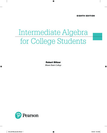
0.1 Basic Set Theory and Interval Notation5UCosmlkaeiuSVA Venn Diagram for C, S and V .In the Venn Diagram above we have three circles - one for each of the sets C, S and V . Wevisualize the area enclosed by each of these circles as the elements of each set. Here, we’vespelled out the elements for definitiveness. Notice that the circle representing the set C is completely inside the circle representing S. This is a geometric way of showing that C S. Also,notice that the circles representing S and V overlap on the letter ‘o’. This common region is howwe visualize S V . Notice that since C V , the circles which represent C and V have nooverlap whatsoever.All of these circles lie in a rectangle labeled U (for ‘universal’ set). A universal set contains allof the elements under discussion, so it could always be taken as the union of all of the sets inquestion, or an even larger set. In this case, we could take U S V or U as the set of lettersin the entire alphabet. The reader may well wonder if there is an ultimate universal set whichcontains everything. The short answer is ‘no’ and we refer you once again to Russell’s Paradox.The usual triptych of Venn Diagrams indicating generic sets A and B along with A B and A Bis given below.UUUA BABSets A and B.AA BBA B is shaded.ABA B is shaded.

6Prerequisites0.1.2Sets of Real NumbersThe playground for most of this text is the set of Real Numbers. Many quantities in the ‘real world’can be quantified using real numbers: the temperature at a given time, the revenue generatedby selling a certain number of products and the maximum population of Sasquatch which caninhabit a particular region are just three basic examples. A succinct, but nonetheless incomplete5definition of a real number is given below.Definition 0.6. A real number is any number which possesses a decimal representation. Theset of real numbers is denoted by the character R.Certain subsets of the real numbers are worthy of note and are listed below. In fact, in moreadvanced texts,6 the real numbers are constructed from some of these subsets.Special Subsets of Real Numbers1. The Natural Numbers: N {1, 2, 3, .} The periods of ellipsis ‘.’ here indicate that thenatural numbers contain 1, 2, 3 ‘and so forth’.2. The Whole Numbers: W {0, 1, 2, .}.3. The Integers: Z {. , 3, 2, 1, 0, 1, 2, 3, .} {0, 1, 2, 3, .}.a 4. The Rational Numbers: Q ba a Z and b Z . Rational numbers are the ratios ofintegers where the denominator is not zero. It turns out that another way to describe therational numbersb is:Q {x x possesses a repeating or terminating decimal representation}5. The Irrational Numbers: P {x x R but x / Q}.c That is, an irrational number is areal number which isn’t rational. Said differently,P {x x possesses a decimal representation which neither repeats nor terminates}aThe symbol is read ‘plus or minus’ and it is a shorthand notation which appears throughout the text. Justremember that x 3 means x 3 or x 3.bSee Section 9.2. cExamples here include number π (See Section 10.1), 2 and 0.101001000100001 .Note that every natural number is a whole number which, in turn, is an integer. Each integer is arational number (take b 1 in the above definition for Q) and since every rational number is a realnumber7 the sets N, W, Z, Q, and R are nested like Matryoshka dolls. More formally, these setsform a subset chain: N W Z Q R. The reader is encouraged to sketch a Venn Diagramdepicting R and all of the subsets mentioned above. It is time for an example.5Math pun intended!See, for instance, Landau’s Foundations of Analysis.7Thanks to long division!6

0.1 Basic Set Theory and Interval Notation7Example 0.1.1.1. Write a roster description for P {2n n N} and E {2n n Z}.2. Write a verbal description for S {x 2 x R}.3. Let A { 117, 45 , 0.202002, 0.202002000200002 .}.(a) Which elements of A are natural numbers? Rational numbers? Real numbers?(b) Find A W, A Z and A P.4. What is another name for N Q? What about Q P?Solution.1. To find a roster description for these sets, we need to list their elements. Starting withP {2n n N}, we substitute natural number values n into the formula 2n . For n 1 we get21 2, for n 2 we get 22 4, for n 3 we get 23 8 and for n 4 we get 24 16. Hence Pdescribes the powers of 2, so a roster description for P is P {2, 4, 8, 16, .} where the ‘.’indicates the that pattern continues.8Proceeding in the same way, we generate elements in E {2n n Z} by plugging in integervalues of n into the formula 2n. Starting with n 0 we obtain 2(0) 0. For n 1 we get2(1) 2, for n 1 we get 2( 1) 2 for n 2, we get 2(2) 4 and for n 2 we get2( 2) 4. As n moves through the integers, 2n produces all of the even integers.9 A rosterdescription for E is E {0, 2, 4, .}.2. One way to verbally describe S is to say that S is the ‘set of all squares of real numbers’.While this isn’t incorrect, we’d like to take this opportunity to delve a little deeper.10 Whatmakes the set S {x 2 x R} a little trickier to wrangle than the sets P or E above is thatthe dummy variable here, x, runs through all real numbers. Unlike the natural numbers orthe integers, the real numbers cannot be listed in any methodical way.11 Nevertheless, wecan select some real numbers, square them and get a sense of what kind of numbers lie in 2S. For x 2, x 2 ( 2)2 4 so 4 is in S, as are 23 94 and ( 117)2 117. Even thingslike ( π)2 and (0.101001000100001 .)2 are in S.So suppose s S. What can be said about s? We know there is some real number x sothat s x 2 . Since x 2 0 for any real number x, we know s 0. This tells us that everything8This isn’t the most precise way to describe this set - it’s always dangerous

COLLEGE ALGEBRA VERSION bˇc PENN STATE ALTOONA – MATH 021 EDITION1 BY Carl Stitz, Ph.D. Jeff Zeager, Ph.D. Lakeland Community College Lorain County Community College Fall 2016 1This is a shorter and slightly modified version of the original manuscript.It only covers the material from chapters 0, 1, and 2,