Transcription
Introductory Quantum ChemistryChem 570a: Lecture NotesProf. Victor S. BatistaRoom: Sterling Chemistry Laboratories (SCL) 19Tuesdays and Thursdays 9:00 – 10:15 amYale University - Department of Chemistry1
Contents1Syllabus72The Fundamental Postulates of Quantum Mechanics3Continuous Representations114Vector SpaceExercise 1 . . . . . . . . . . . . . . . . . . . . . . . . . . . . . . . . . . . . . . .Exercise 2 . . . . . . . . . . . . . . . . . . . . . . . . . . . . . . . . . . . . . . .1114145Stationary States5.1 Exercise 3 . . . . . . . . . . . . . . . . . . . . . . . . . . . . . . . . . . . . . . .5.2 Exercise 4 . . . . . . . . . . . . . . . . . . . . . . . . . . . . . . . . . . . . . . .5.3 Exercise 5 . . . . . . . . . . . . . . . . . . . . . . . . . . . . . . . . . . . . . . .151515166Particle in the Box6.1 Exercise 6 . . . . . . . . . . . . . . . . . . . . . . . . . . . . . . . . . . . . . . .16177Commutator7.1 Exercise 7 . . . . . . . . . . . . . . . . . . . . . . . . . . . . . . . . . . . . . . .18188Uncertainty Relations8.1 Exercise 8 . . . . . . . . . . . . . . . . . . . . . . . . . . . . . . . . . . . . . . .8.2 EPR Paradox . . . . . . . . . . . . . . . . . . . . . . . . . . . . . . . . . . . . .1819199Exercise 99.1 Copenhagen Interpretation:9.2 Feynman Interview: . . . .9.3 Momentum Operator: . . .9.4 EPR Paradox: . . . . . . .9.5 Schrödinger’s cat paradox:2020202021214.14.2.8.10 Heisenberg Representation1121Fourier Grid Hamiltonian11.1 Computational Problem FGH . . . . . . . . . . . . . . . . . . . . . . . . . . . . .242512 Variational Theorem2513 Digital Grid-Based Representations13.1 Computational Problem 1 . . . . . . . . . . . . . . . . . . . . . . . . . . . . . . .13.2 Computational Problem 2 . . . . . . . . . . . . . . . . . . . . . . . . . . . . . . .2727282
13.3 Computational Problem 3 . . . . . . . . . . . . . . . . . . . . . . . . . . . . . . .13.4 Computational Problem 4 . . . . . . . . . . . . . . . . . . . . . . . . . . . . . . .14 SOFT Method14.1 Computational Problem 5 . . . . . . . . . . .14.2 Imaginary time propagation . . . . . . . . . .14.3Ehrenfest Dynamics . . . . . . . .14.4 Exercise: Real and Imaginary Time Evolution14.5 Computational Problem 6 . . . . . . . . . . .14.6 Computational Problem 7 . . . . . . . . . . .14.7 Computational Problem 8 . . . . . . . . . . .14.8 Computational Problem 9 . . . . . . . . . . .2929.30303132333435353515 Time Independent Perturbation Theory15.1 Exercise 9: How accurate is first order time-independent perturbation theory?353616 Time Dependent Perturbation Theory16.1 Exercise 10 . . . . . . . . . . . . . . . . . . . . . . . . . . . . . . . . . . . . . .16.2 Exercise 11 . . . . . . . . . . . . . . . . . . . . . . . . . . . . . . . . . . . . . .37404117.Golden Rule4317.1 Monochromatic Plane Wave . . . . . . . . . . . . . . . . . . . . . . 4317.2 Vibrational Cooling . . . . . . . . . . . . . . . . . . . . . . . . . . . . . . . . . .17.3Electron Transfer . . . . . . . . . . . . . . . . . . . . . . . . . . . . . .18 Problem Set18.1 Exercise 11 . . . . . . . . . . . . . . . . . . . . . . . .18.2 Exercise 12 . . . . . . . . . . . . . . . . . . . . . . . .18.3 Exercise 13 . . . . . . . . . . . . . . . . . . . . . . . .18.4 Exercise 14 . . . . . . . . . . . . . . . . . . . . . . . .18.5 Time Evolution Operator . . . . . . . . . . . . . . . . .18.5.1 Evolution in the basis of eigenstates: . . . . . . .18.5.2 Trotter expansion of the time evolution operator:18.5.3 Numerical Comparison: . . . . . . . . . . . . .444749494950515151515119 Adiabatic Approximation5220 Two-Level Systems5321 Harmonic Oscillator21.1 Exercise 15 . . . . . . . . . . . . . . . . . . . . . . . . . . . . . . . . . . . . . .21.2 Exercise: Analytical versus SOFT Propagation . . . . . . . . . . . . . . . . . . .5757603
22 Problem Set22.1 Exercise 16 . . . . . . . . . . .22.2 Exercise 17 . . . . . . . . . . .22.3 Exercise 18 . . . . . . . . . . .22.4 Exercise 19 . . . . . . . . . . .22.5 Exercise 20: Morse Oscillator .616162626263.656668707071.747677777825 Central Potential25.1 Exercise 30 . . . . . . . . . . . . . . . . . . . . . . . . . . . . . . . . . . . . . .798126 Two-Particle Rigid-Rotor26.1 Exercise 31 . . . . . . . . . . . . . . . . . . . . . . . . . . . . . . . . . . . . . .828227 Problem Set27.1 Exercise 3227.2 Exercise 3327.3 Exercise 3427.4 Exercise 3527.5 Exercise 3627.6 Exercise 37.8282828283838328 Hydrogen Atom28.1 Exercise 3828.2 Exercise 3928.3 Exercise 4028.4 Exercise 4128.5 Exercise 42.83858686868723 Angular Momentum23.1 Exercise 21 . .23.2 Exercise 22 . .23.3 Exercise 23 . .23.4 Exercise 24 . .23.5 Exercise 25 . .24 Spin Angular Momentum24.1 Exercise 26 . . . . .24.2 Exercise 27 . . . . .24.3 Exercise 28 . . . . .24.4 Exercise 29 . . . . .29 Helium Atom.884
30 Spin-Atom Wavefunctions8931 Pauli Exclusion Principle9032 Lithium Atom32.1 Exercise 44 . . . . . . . . . . . . . . . . . . . . . . . . . . . . . . . . . . . . . .919233 Spin-Orbit Interaction33.1 Exercise 45 . . . . . . . . . . . . . . . . . . . . . . . . . . . . . . . . . . . . . .929434 Periodic Table34.1 Exercise 46 . . . . . . . . . . . . . . . . . . . . . . . . . . . . . . . . . . . . . .34.2 Exercise 47 . . . . . . . . . . . . . . . . . . . . . . . . . . . . . . . . . . . . . .94969635 Problem Set35.1 Exercise 4835.2 Exercise 4935.3 Exercise 5035.4 Exercise 519696979797.36 LCAO Method: H 972 Molecule36.1 Exercise 52 . . . . . . . . . . . . . . . . . . . . . . . . . . . . . . . . . . . . . . 9836.2 Exercise 53 . . . . . . . . . . . . . . . . . . . . . . . . . . . . . . . . . . . . . . 10037 H2 Molecule10137.1 Heitler-London(HL) Method: . . . . . . . . . . . . . . . . . . . . . . . . . . . . 10337.2 Exercise 54 . . . . . . . . . . . . . . . . . . . . . . . . . . . . . . . . . . . . . . 10338 Homonuclear Diatomic Molecules10338.1 Exercise 55 . . . . . . . . . . . . . . . . . . . . . . . . . . . . . . . . . . . . . . 10739 Conjugated Systems: Organic Molecules10840 Self-Consistent Field Hartree-Fock Method11040.1 Restricted Closed Shell Hartree-Fock . . . . . . . . . . . . . . . . . . . . . . . . 11440.2 Configuration Interaction . . . . . . . . . . . . . . . . . . . . . . . . . . . . . . 11840.3 Supplement: Green’s Function . . . . . . . . . . . . . . . . . . . . . . . . . . . 11841Second Quantization Mapping41.141.241.341.441.5Single-Particle Basis . . . . . . . . . .Occupation Number Basis . . . . . . .Creation and Anihilation Operators . . .Operators in Second Quantization . . .Change of basis in Second Quantization5.123123124124125127
41.6 Mapping into Cartesian Coordinates . . . . . . . . . . . . . . . . . . . . . . . . . 12742Density Functional Theory42.142.242.342.4Hohenberg and Kohn TheoremsKohn Sham Equations . . . . .Thomas-Fermi Functional . . .Local Density Approximation .43 Quantum Mechanics/Molecular Mechanics Methods12913113213313413644 Empirical Parametrization of Diatomic Molecules13744.1 Exercise 56 . . . . . . . . . . . . . . . . . . . . . . . . . . . . . . . . . . . . . . 14044.2 Exercise 57 . . . . . . . . . . . . . . . . . . . . . . . . . . . . . . . . . . . . . . 14145Discrete Variable Representation14345.1 Multidimensional DVR . . . . . . . . . . . . . . . . . . . . . . . . . . . . . . . . 14645.2 Computational Problem 15 . . . . . . . . . . . . . . . . . . . . . . . . . . . . . . 14646 Tunneling Current: Landauer Formula14746.1 WKB Transmission . . . . . . . . . . . . . . . . . . . . . . . . . . . . . . . . . . 15047Solutions to Computational blem 1Problem 2Problem 3Problem 4Problem 5Problem 6Problem 7Problem 8Problem 9.6.153153156161164170171182200217
1 SyllabusThe goal of this course is to introduce fundamental concepts of Quantum Mechanics with emphasison Quantum Dynamics and its applications to the description of molecular systems and their interactions with electromagnetic radiation. Quantum Mechanics involves a mathematical formulationand a physical interpretation, establishing the correspondence between the mathematical elementsof the theory (e.g., functions and operators) and the elements of reality (e.g., the observable properties of real systems).1 The presentation of the theory will be mostly based on the so-called OrthodoxInterpretation, developed in Copenhagen during the first three decades of the 20th century. However, other interpretations will be discussed, including the ’pilot-wave’ theory first suggested byPierre De Broglie in 1927 and independently rediscovered by David Bohm in the early 1950’s.Textbooks: The official textbook for this class is:R1: Levine, Ira N. Quantum Chemistry; 5th Edition; Pearson/Prentice Hall; 2009.However, the lectures will be heavily complemented with material from other textbooks including:R2: ”Quantum Theory” by David Bohm (Dover),R3: ”Quantum Physics” by Stephen Gasiorowicz (Wiley),R4: ”Quantum Mechanics” by Claude Cohen-Tannoudji (Wiley Interscience),R5: ”Quantum Mechanics” by E. Merzbacher (Wiley),R6: ”Modern Quantum Mechanics” by J. J. Sakurai (Addison Wesley),All these references are ’on-reserve’ at the Kline science library.References to specific pages of the textbooks listed above are indicated in the notes as follows:R1(190) indicates “for more information see Reference 1, Page 190”.Furthermore, a useful mathematical reference is R. Shankar, Basic Training in Mathematics. AFitness Program for Science Students, Plenum Press, New York 1995.Useful search engines for mathematical and physical concepts can be found athttp://scienceworld.wolfram.com/physics/ and http://mathworld.wolfram.com/The lecture notes are posted online at: (http://ursula.chem.yale.edu/ batista/classes/vvv/v570.pdf)Grading: Grading and evaluation is the same for both undergraduate and graduate students. Themid-terms will be on 10/12 and 11/07. The date for the Final Exam is determined by Yale’s calendarof final exams. Homework includes exercises and computational assignments due one week afterassigned.Contact Information and Office Hours: Prof. Batista will be glad to meet with studentsat SCL 115 as requested by the students via email to victor.batista@yale.edu, or by phone at (203)432-6672.1Old Story: Heisenberg and Schrödinger get pulled over for speeding. The cop asks Heisenberg ”Do you know howfast you were going?” Heisenberg replies, ”No, but we know exactly where we are!” The officer looks at him confusedand says ”you were going 108 miles per hour!” Heisenberg throws his arms up and cries, ”Great! Now we’re lost!”The officer looks over the car and asks Schröinger if the two men have anything in the trunk. ”A cat,” Schrödingerreplies. The cop opens the trunk and yells ”Hey! This cat is dead.” Schrödinger angrily replies, ”Well he is now.”7
2The Fundamental Postulates of Quantum MechanicsQuantum Mechanics can be formulated in terms of a few postulates (i.e., theoretical principlesbased on experimental observations). The goal of this section is to introduce such principles, together with some mathematical concepts that are necessary for that purpose. To keep the notationas simple as possible, expressions are written for a 1-dimensional system. The generalization tomany dimensions is usually straightforward.P ostulate 1 : Any system in a pure state can be described by a wave-function , ψ(t, x), where t isa parameter representing the time and x represents the coordinates of the system. Such a functionψ(t, x) must be continuous, single valued and square integrable.Note 1: As a consequence of Postulate 4, we will see that P (t, x) ψ (t, x)ψ(t, x)dx representsthe probability of finding the system between x and x dx at time t, first realized by Max Born. 2P ostulate 2 : Any observable (i.e., any measurable property of the system) can be described byan operator. The operator must be linear and hermitian.What is an operator ? What is a linear operator ? What is a hermitian operator?Definition 1: An operator Ô is a mathematical entity that transforms a function f (x) into anotherfunction g(x) as follows, R4(96)Ôf (x ) g(x ),where f and g are functions of x.Definition 2: An operator Ô that represents an observable O is obtained by first writing the classical expression of such observable in Cartesian coordinates (e.g., O O(x, p)) and then substituting the coordinate x in such expression by the coordinate operator x̂ as well as the momentum pby the momentum operator p̂ i / x.Definition 3: An operator Ô is linear if and only if (iff),Ô(af (x) bg(x)) aÔf (x) bÔg(x),where a and b are constants.Definition 4: An operator Ô is hermitian iff, Z Z dxψm (x)Ôφn (x) ,dxφn (x)Ôψm (x) 2Note that this probabilistic interpretation of ψ has profound implications to our understanding of reality. It essentially reduces the objective reality to P (t, x). All other properties are no longer independent of the process ofmeasurement by the observer. A. Pais’ anecdote of his conversation with A. Einstein while walking at Princeton emphasizes the apparent absurdity of the implications: [Rev. Mod. Phys. 51, 863914 (1979), p. 907]: ’We often discussedhis notions on objective reality. I recall that during one walk Einstein suddenly stopped, turned to me and asked whetherI really believed that the moon exists only when I look at it.’8
where the asterisk represents the complex conjugate.Definition 5: A function φn (x) is an eigenfunction of Ô iff,Ôφn (x) On φn (x),where On is a number called eigenvalue.Property 1: The eigenvalues of a hermitian operator are real.Proof: Using Definition 4, we obtain ZZ dxφn (x)Ôφn (x) 0,dxφn (x)Ôφn (x) therefore,[On On ]Zdxφn (x) φn (x) 0.Since φn (x) are square integrable functions, then,On On .Property 2: Different eigenfunctions of a hermitian operator (i.e., eigenfunctions with differenteigenvalues) are orthogonal (i.e., the scalar product of two different eigenfunctionsis equal toRzero). Mathematically, if Ôφn On φn , and Ôφm Om φm , with On 6 Om , then dxφ n φm 0.Proof: Z Zdxφ m Ôφn andZ[On Om ]Since On 6 Om , thendxφ n ÔφmR 0,dxφ m φn 0.dxφ m φn 0.P ostulate 3 : The only possible experimental results of a measurement of an observable are theeigenvalues of the operator that corresponds to such observable.P ostulate 4 : The average value of many measurements of an observable O, when the system isdescribed by ψ(x) as equal to the expectation value Ō, which is defined as follows,Rdxψ(x) Ôψ(x)Ō R.dxψ(x) ψ(x)P ostulate 5 :The evolution of ψ(x, t) in time is described by the time-dependent Schrödingerequation :9
i 2 ψ(x, t) Ĥψ(x, t), t2 where Ĥ 2m V̂ (x), is the operator associated with the total energy of the system, E x22p V (x).2mExpansion P ostulate : R5(15), R4(97)The eigenfunctions of a linear and hermitian operator form a complete basis set. Therefore,any function ψ(x) that is continuous, single valued, and square integrable can be expanded as alinear combination of eigenfunctions φn (x) of a linear and hermitian operator  as follows,Xψ(x) Cj φj (x),jwhere Cj are numbers(e.g., complex numbersP ) called expansion coefficients.P Note that Ā j Cj Cj aj , when ψ(x) j Cj φj (x),ZÂφj (x) aj φj (x),anddxφj (x) φk (x) δjk .This is because the eigenvalues aj are the only possible experimental results of measurements of Â(according to Postulate 3), and the expectation value Ā is the Paverage value of many measurementsof  when the system is described by the expansion ψ(x) j Cj φj (x) (Postulate 4). Therefore,the product Cj Cj can be interpreted as the probability weight associated with eigenvalue aj (i.e.,the probability that the outcome of an observation of  will be aj ).Hilbert-SpaceAccording to the Expansion Postulate (together with Postulate 1), the state of a system describedby the function Ψ(x) can be expanded as a linear combination of eigenfunctions φj (x) of a linearand hermitian operator (e.g., Ψ(x) C1 φ1 (x) C2 φ2 (x) . . .). Usually, the space defined bythese eigenfunctions (i.e., functions that are continuous, single valued and square integrable) hasan infinite number of dimensions. Such space is called Hilbert-Space in honor to the mathematicianHilbert who did pioneer work in spaces of infinite dimensionality.R4(94)A representation of Ψ(x) in such space of functions corresponds to a vector-function,φ2 (x)6C2.ψ(x) .C1-φ1 (x)10
where C1 and C2 are the projections of Ψ(x) along φ1 (x) and φ2 (x), respectively. All othercomponents are omitted from the representation because they are orthogonal to the “plane” definedby φ1 (x) and φ2 (x).3Continuous RepresentationsCertain operators have a continuous spectrum of eigenvalues. For example, the coordinate operatoris one such operator since it satisfies the equation x̂ δ(x0 x) x0 δ(x0 x), where the eigenvaluesx0 define a continuum. Delta functions δ(x0 x) thus define a continuous representation (the socalled ’coordinate representation’) for whichZψ(x) dx0 Cx0 δ(x0 x),where Cx0 ψ(x0 ), sinceZZZdxδ(x β)ψ(x) dx dαCα δ(x β)δ(α x) ψ(β).When combined with postulates 3 and 4, the definition of the expansion coefficients Cx0 ψ(x0 ) implies that the probability of observing the system with coordinate eigenvalues between x0and x0 dx0 is P (x0 ) Cx0 Cx 0 dx0 ψ(x0 )ψ(x0 ) dx0 (see Note 1).In general, eigenstates φ(α, x) with a continuum spectrum of eigenvalues α define continuousrepresentations,Zψ(x) dαCα φ(α, x),Rwith Cα dxφ(α, x) ψ(x). Delta functions and the plane waves are simply two particularexamples of basis sets with continuum spectra.Note 2: According to the Expansion Postulate, a function ψ(x) is uniquely and completely definedby the coefficients Cj , associated with its expansion in a complete set of eigenfunctions φj (x).However, the coefficients of such expansion would be different if the same basis functions φjdepended on different coordinates (e.g., φj (x0 ) with x0 6 x). In order to eliminate such ambiguityin the description it is necessary to introduce the concept of vector-ket space.R4(108)4Vector SpaceVector-Ket Space ε: The vector-ket space is introduced to represent states in a convenient spaceof vectors φj , instead of working in the space of functions φj (x). The main difference is thatthe coordinate dependence does not need to be specified when working in the vector-ket space.According to such representation, function ψ(x) is the component of vector ψ associated with11
Pindex x (vide infra). Therefore, for any function ψ(x) j Cj φj (x), we can define a ket-vector ψ such that,X ψ Cj φj .jThe representation of ψ in space ε is,Ket-Space ε φ2 6C2. . ψ .C1- φ1 Note that the expansion coefficients Cj depend only on the kets ψj and not on any specificvector component. Therefore, the ambiguity mentioned above is removed.In order to learn how to operate with kets we need to introduce the bra space and the concept oflinear functional. After doing so, this section will be concluded with the description of Postulate5, and the Continuity Equation.Linear functionalsA functional χ is a mathematical operation that transforms a function ψ(x) into a number. Thisconcept is extended to the vector-ket space ε, as an operation that transforms a vector-ket into anumber as follows,χ(ψ(x)) n,orχ( ψ ) n,where n is a number. A linear functional satisfies the following equation,χ(aψ(x) bf (x)) aχ(ψ(x)) bχ(f (x)),where a and b are constants.Example: The scalar product,R4(110)Zn dxψ (x)φ(x),is an example of a linear functional, since such an operation transforms a function φ(x) into anumber n. In order to introduce the scalar product of kets, we need to introduce the bra-space.Bra Space ε : For every ket ψ we define a linear functional ψ , called bra-vector, as follows:R ψ ( φ ) dxψ (x)φ(x).12
Note that functional ψ is linear because the scalar product is a linear functional. Therefore, ψ (a φ b f ) a ψ ( φ ) b ψ ( f ).Note: For convenience, we will omit parenthesis so that the notation ψ ( φ ) will be equivalentto ψ φ . Furthermore, whenever we find two bars next to each other we can merge them intoa single one without changing the meaning of the expression. Therefore, ψ φ ψ φ .P The space of bra-vectors is called dual spaceεsimplybecausegivenaket ψ j Cj φj ,P the corresponding bra-vector is ψ j Cj φj . In analogy to the ket-space, a bra-vector ψ is represented in space ε according to the following diagram:Dual-Space ε φ2 6C2 . . ψ . C1- φ1 where Cj is the projection of ψ along φj .Projection Operator and Closure RelationGiven a ket ψ in a certain basis set φj , ψ XCj φj ,(1)jwhere φk φj δkj ,Cj φj ψ .(2)Substituting Eq. (2) into Eq.(1), we obtain ψ X φj φj ψ .jFrom Eq.(3), it is obvious thatX φj φj 1̂,Closure Relationj13(3)
where 1̂ is the identity operator that transforms any ket, or function, into itself.Note that P̂j φj φj is an operator that transforms any vector ψ into a vector pointingin the direction of φj with magnitude φj ψ . The operator P̂j is called the ProjectionOperator. It projects φj according to,P̂j ψ φj ψ φj .Note that P̂j2 P̂j , where P̂j2 P̂j P̂j . This is true simply because φj φj 1.4.1Exercise 1Prove thati P̂j [Ĥ, P̂j ], twhere [Ĥ, P̂j ] Ĥ P̂j P̂j Ĥ.Continuity Equation4.2Exercise 2Prove thatwhere (ψ (x, t)ψ(x, t)) j(x, t) 0, t x ψ(x, t) ψ (x, t) ψ (x, t) ψ(x, t).j(x, t) 2mi x xIn general, for higher dimensional problems, the change in time of probability density, ρ(x, t) ψ (x, t)ψ(x, t), is equal to minus the divergence of the probability flux j, ρ(x, t) · j. tThis is the so-called Continuity Equation .Note: Remember that given a vector field j, e.g., j(x, y, z) j1 (x, y, z)î j2 (x, y, z)ĵ j3 (x, y, z)k̂, the divergence of j is defined as the dot product of the “del” operator ( x, y, z) and vector jas follows: j1 j2 j3 ·j . x y z14
5Stationary StatesStationary states are states for which the probability density ρ(x, t) ψ (x, t)ψ(x, t) is constantat all times (i.e., states for which ρ(x,t) 0, and therefore · j 0). In this section we will show tthat if ψ(x, t) is factorizable according to ψ(x, t) φ(x)f (t), then ψ(x, t) is a stationary state.Substituting ψ(x, t) in the time dependent Schrödinger equation we obtain:φ(x)i 2 2 φ(x) f (t) f (t) f (t)V (x)φ(x), t2m x2and dividing both sides by f (t)φ(x) we obtain: 2 2 φ(x)i f (t) V (x).f (t) t2mφ(x) x2(4)Since the right hand side (r.h.s) of Eq. (4) can only be a function of x and the l.h.s. can only be afunction of t for any x and t, and both functions have to be equal to each other, then such functionmust be equal to a constant E. Mathematically,ii f (t) E f (t) f (0)exp( Et),f (t) t 2 2 φ(x) V (x) E Ĥφ(x) Eφ(x) .2mφ(x) x2The boxed equation is called the time independent Schrödinger equation.Furthermore, since f (0) is a constant, function φ̃(x) f (0)φ(x) also satisfies the time independentSchrödinger equation as follows,Ĥ φ̃(x) E φ̃(x) ,andiψ(x, t) φ̃(x)exp( Et). Eq. (5) indicates that E is the eigenvalue of Ĥ associated with the eigenfunction φ̃(x).5.1Exercise 3Prove that Ĥ is a Hermitian operator.5.2Exercise 4Prove that -i / x is a Hermitian operator.15(5)
5.3Exercise 5Prove that if two hermitian operators Q̂ and P̂ satisfy the equation Q̂P̂ P̂ Q̂, i.e., if P and Qcommute (vide infra), the product operator Q̂P̂ is also hermitian.Since Ĥ is hermitian, E is a real number E E (see Property 1 of Hermitian operators), then,ψ (x, t)ψ(x, t) φ̃ (x)φ̃(x). Since φ̃(x) depends only on x, t(φ̃ (x)φ̃(x)) 0, then, tψ (x, t)ψ(x, t) 0. This demonstrationproves that if ψ(x, t) φ(x)f (t), then ψ(x, t) is a stationary function.6Particle in the BoxThe particle in the box can be represented by the following diagram:R1(22)V (x) Box66V V V 0r- xa0ParticleThe goal of this section is to show that a particle with energy E and mass m in the box-potentialV(x) defined as(0,when 0 x a,V (x) ,otherwise,has stationary states and a discrete absorption spectrum (i.e., the particle absorbs only certaindiscrete values of energy called quanta). To that end, we first solve the equation Ĥ φ̃(x) E φ̃(x),and then we obtain the stationary states ψ(x, t) φ̃(x)exp( i Et).Since φ̃(x) has to be continuous, single valued and square integrable (see Postulate 1), φ̃(0) andφ̃(a) must satisfy the appropriate boundary conditions both inside and outside the box. The boundary conditions inside the box lead to: 2 Φ(x) EΦ(x),2m x2 Φ(x) A Sin(K x).(6)Functions Φ(x) determine the stationary states inside the box. The boundary conditions outside thebox are, 2 Φ(x) Φ(x) EΦ(x), Φ(x) 0,2m x216
and determine the energy associated with Φ(x) inside the box as follows. From Eq. (6), we obtain: 2AK 2 EA, and, Φ(a) ASin(K a) 0,2m Ka nπ, with n 1, 2, . Note that the number of nodes of Φ (i.e., the number of coordinates where Φ(x) 0), is equal ton 1 for a given energy, and the energy levels are,E 2 n2 π 2,2m a2with n 1, 2, .e.g., 2 π 2,2m a2 2 4π 2E(n 2) , .2m a2Conclusion: The energy of the particle in the box is quantized! (i.e., the absorption spectrum ofthe particle in the box is not continuous but discrete).E(n 1) 6.1Exercise 6(i) Using the particle in the box model for an electron in a quantum dot (e.g., a nanometer sizesilicon material) explain why larger dots emit in the red end of the spectrum, and smaller dots emitblue or ultraviolet.(ii) Consider the molecule hexatriene CH2 CH CH CH CH CH2 and assume thatthe 6 π electrons move freely along the molecule. Approximate the energy levels using the particlein the box model. The length of the box is the sum of bond lengths with C-C 1.54 Å, C C 1.35Å, and an extra 1.54 Å, due to the ends of the molecule. Assume that only 2 electrons can occupyeach electronic state and compute:(A) The energy of the highest occupied energy level.(B) The energy of the lowest unoccupied energy level.17
(C) The energy difference between the highest and the lowest energy levels, and compare suchenergy difference with the energy of the peak in the absorption spectrum at λM AX 268nm.(D) Predict whether the peak of the absorption spectrum for CH2 CH (CH CH)n CH CH2 would be red- or blue-shifted relative to the absorption spectrum of hexatriene.7CommutatorThe commutator [Â, B̂] is defined as follows:R4(97)[Â, B̂] ÂB̂ B̂ Â.Two operators  and B̂ are said to commute when [Â, B̂] 0.7.1Exercise 7 ] i . Hint: Prove that [x̂, i x]ψ(x) i ψ(x), where ψ(x) is a functionProve that [x̂, i xof x.Note: Mathematically, we see that the momentum and position operators do not commute simplybecause p̂ i / x, so p̂x i (1 x / x) is not the same as xp̂ i x / x. Conceptually,it means that one cannot measure the position without affecting the state of motion since measuringthe position would perturb the momentum. To measure the position of a particle it is necessaryto make it leave a mark on a sensor/detector (e.g., a piece chalk needs to leave a mark on theblackboard to report its position). That process unavoidably slows it down, affecting its momentum.8Uncertainty RelationsqThe goal of this section is to show that the uncertainties A (  )2 and B q (B̂ B̂ )2 , of any pair of hermitian operators  and B̂, satisfy the uncertainty relation:R3(437)1( A)2 ( B)2 i[A, B] 2 .(7)4In particular, when  x̂ and B̂ p̂, we obtain the Heisenberg uncertainty relation : x · p Proof:Û Â A ,V̂ B̂ B , .2φ(λ, x) R (Û iλV̂ )Φ(x),I(λ) dxφ (λ, x)φ(λ, x) 0,18(8)
ZI(λ) dx[(Â A )Φ(x) iλ(B̂ B )
Quantum Mechanics involves a mathematical formulation and a physical interpretation, establishing the correspondence between the mathematical elements of the theory (e.g., functions and operators)