Transcription
Paper 2831-2018Evaluating the accuracy of clinical prediction models for binary and survival outcomesJoseph C. Gardiner, Department of Epidemiology and Biostatistics,Michigan State University, East Lansing, MI 48824AbstractClinical prediction models employ regression-based methods to elucidate potential predictors ofoutcomes. For a binary outcome, the LOGISTIC and HPLOGISTIC procedures offer options formodel development, testing and validation. Several fit statistics can be used to gauge the predictiveaccuracy of a model as well as for comparisons between competing models. In the appropriate contextthese statistics include sensitivity, specificity, positive and negative predictive values, the receiveroperating characteristic (ROC) curve and concordance indices. A similar development for survivalmodels faces many challenges, including the feature of time-dependent outcome and censoring inaccrued survival data. New options in the PHREG procedure permit calculation of some of theaforementioned fit statistics. We discuss their interpretation and illustrate their application with empiricaldata sets.1. IntroductionClinical prediction models are ubiquitous in medicine (Steyerberg, 2009). Prediction models have at theircore a diagnostic marker based on contemporaneous and antecedent variables that can predict thelikelihood of a future random event. Khorana et al (2008) develop a prediction rule for the risk of venousthromboembolism (VTE) in cancer patients on active chemotherapy. A single-index is constructed frombaseline clinical and laboratory assessments that could help identify patients at high risk of VTE so thatprophylaxis could be initiated. Gardiner et al (2016) report on the incidence of hospital-acquired pressureulcers in a population-based retrospective cohort. The objective was to assess the relative importance ofpatient variables such as gender, race, age, comorbidities, body mass index in identifying patients whomight be at higher risk of acquiring a pressure ulcer during their hospital stay.From studies in which the event outcome and its potential correlates are available, a series of prognosismodels can be evaluated with respect to their discriminative ability. Their common structure models thepresence of disease ( D 1) from potential predictor variables x through a logistic regression model,P[ D 1 x ] (1 exp( x′β )) . From the distribution of the single index M x′β , the sensitivity 10] can be compared by varying the cut-off value c.P[ M c D 1] and specificity P[ M c D Sensitivity is called the true positive ratio TP ( c ) and 1 minus specificity, the false positive ratio FP ( c ) . Thereceiver operating characteristic (ROC) curve is a display of the points ( FP ( c ), TP ( c )) for varying cut-offsthat could aid in a judicious choice of c. The area under the ROC curve (AUC) is a summary statisticcalled the c-statistic. It has an interpretation as the probability that the marker for a randomly selectedsubject from the diseased population ( D 1) is greater than the marker for a randomly selected subjectfrom the non-diseased population ( D 0) . Since these statistics depend on x, one can assess competinglogistic models with different covariate sets in their ability to provide a relatively simpler discriminationbetween true positive and false positive ratios. For example, a c-statistic above 0.75 is consideredexcellent. Sub-models with fewer covariates may be compared with respect to their c-statistics.1
Paper 2831-2018For a binary outcome, the LOGISTIC procedure is the workhorse for estimating the logistic model.Options for ROC analyses of competing models and statistical comparisons between them are available.Both LOGISITC and HPLOGISTIC provide a scheme for development, testing and validation of theprediction model.Survival outcomesWe begin with a time-to-event T measured from origin t 0 and a marker M measured at baseline.Higher values of the marker are indicative of worse prognosis for the event. Potential predictor variablesx ) P[ T t x ] can be assessed using the semiparametric Coxx of the survival distribution S ( t proportional hazards model (PHM) h( t x ) h0 ( t )exp( x′β ) with baseline hazard function h0 and thesingle index M x′β . An alternative model is the parametric accelerated failure time model (AFT),log T x′β σε with a specified distribution on ε and scale parameter σ ( 0). For example, thex ) exp ( {t / θ ( x )}1/σ ) whereextreme-value distribution for ε corresponds to Weibull survival S ( t log θ ( x ) x′β . In the AFT context we use M x′β to maintain the convention that higher values ofthe marker indicate poorer survival outcome.The next step is to define sensitivity and specificity of the diagnostic marker. Several definitions havebeen proposed (Heagerty and Zhang, 2005, Pepe et al, 2008). PHREG adopts the cumulative/dynamicdefinition:TP ( c , t ) Sensitivity(c, t ) P[ M c T t ] , and Specificity(c, t ) P[ M c T t ] 1 FP ( c , t ) .(1)Interpreting T as the time to disease onset, the definitions are similar to those for a binary outcome, by [ T t ] . With t fixed, the true positive ratio TP ( c , t ) and false positive ratio FP ( c , t ) aretaking Dmonotone decreasing functions of the cut-off c, but not necessarily strictly decreasing. As probabilitiesthey are bounded on [0, 1]. It is desirable for estimators of these quantities to have the same properties.ROC curve and AUCGiven TP ( c , t ) and FP ( c , t ) , the points of the ROC curve are ROC(t) {( FP ( c , t ) , TP ( c , t ) ): c ℜ}.Formally, define ROC(p, t) TP{[ FP ( p , t )] 1 , t } where [ FP ( p , t )] 1 inf{c : FP ( c , t ) p}, p [0,1]} . For1each t, p ROC(p, t) is a function on [0, 1]. The area under the ROC is AUC ( t ) ROC ( p , t )dp .0From independent pairs ( M 1 , T1 ),( M 2 , T2 ) we may interpret AUC ( t ) as(2)AUC ( t ) P[ M 1 M 2 T1 t T2 ]At time t, given that the event has occurred in subject 1, but has not yet occurred in subject 2, AUC ( t )is the probability that the marker M 1 in subject 1 is greater than the marker M 2 in subject 2. It measuresthe ability of the markers to correctly order the event status at time t.Integrated AUCAn ‘average’ AUC ( t ) for all t is obtained as E ( AUC ( T ))2 0AUC ( t )( dS ( t ))
Paper 2831-20182. EstimationWith survival data we must address incomplete observation of the survival outcome, that is, T might be(right) censored. Let {( Ti , δ i , x i ) : 1 i n} denote the observations from a random sample withobserved time Ti min( Ti , C i ) , event time Ti , censoring time C i and (right) censoring indicatorδ [ Ti C i ] . Thus δ i 1 if Ti is an event time, and δ i 0 otherwise. The covariates x i are timeiinvariant and used to define the marker M i x′i β . Estimation of β is via maximum partial likelihood inthe Cox PHM. Minimally, we assume ( Ti , C i ) are conditionally independent given x i , but in much ofwhat follows the censoring distribution is assumed not to depend on x i . In several applications thisassumption may not be tenable (Blanche et al, 2013a). Following historical development of ROCanalyses, PHREG offers four methods of estimation of the quantities TP ( c , t ) , FP ( c , t ) , the ROC curve,ROC(t) and AUC(t).Conditional Kaplan –Meier (METHOD KM)Start with the definitions (1) to obtainM c T t ]TP ( c , t ) P[ P[ T t M c ]P[ M c ] 1 S ( t M c ) (1 FM ( c ))P[ T t ]1 S( t )FP ( c , t ) P[ M c T t ] P[ T t M c ]P[ M c ] S ( t M c )(1 FM ( c )) , P[ T t ]S( t )in terms of the survival distribution S ( t ) P[ T t ] , the conditional survival distribution S ( t M c )and the distribution of the marker FM ( c ) P[ M c ] . Estimation is simple plug-in with the KaplanMeier (KM) estimator of S ( t ) from all data, for S ( t M c ) using only the subsample, and FM ( c )estimated by its empirical cumulative distribution function. This is essentially done in Lu and Liu(2006).The KM estimators of S ( t M c ) are based on different subsamples due to varying cut-off c. Theresulting estimators of TP ( c , t ) and FP ( c , t ) need not be monotone in c and could take values outside[0, 1]. The estimated ROC(t) could also be non-monotone and take values outside the unit square.Heagerty et al (2000) give a numerical example to illustrate this issue. It is not necessarily seen onlywith small to moderate size samples.Inverse-probability of censoring weighted (IPCW) estimator (METHOD IPCW)From definitions (1), TP ( c , t ) P[ T t , M c ]P[ T t , M c ]and FP ( c , t ) . Use plug-in empiricalP[ T t ]P[ T t ]estimates for the numerator and denominator of TP ( c , t ) , but weighted by the inverse probability ofnot being censored at time Ti , which is estimated by SˆC ( Ti ) where SˆC (.) is the KM estimator ofthe censoring distribution, assumed independent of covariates.3
Paper 2831-2018Use the data {( Ti , δ i ) : 1 i n} with LIFETEST regarding censoring times as the response to obtainSˆC (.) . The explicit formulae are (Blanche et al, 2013a):nn[ T t , M i c ]δ i / SˆC ( Ti )[T t , M i c ] i 1 ii 1 i and FP ( c , t ) .TP ( c , t ) nn i 1[Ti t ] i 1[Ti t ]δ i / SˆC (Ti )(3)These IPCW estimators are monotone and bounded on [0. 1]. The weighting scheme was proposed byUno et al (2007) motivated by P[C T T , M ] SC ( T ) which results in δ [T t , M c ] E P[ T t , M c ] . We obtain consistency and asymptotic normality under standardSC ( T ) assumptions (Uno et al, 2007, Hung and Chiang, 2010a). Assume that the censoring distribution does notdepend on the marker M. This is sufficient to demonstrate the convergence in probability, ( c , t ) TP ( c , t ), TPFP ( c , t ) FP ( c , t ). From (3) we also get an estimator AUC ( t ) of AUC ( t ) . Hungand Chiang (2010b) and Blanche et al (2013a) give an explicit expression suggested from U-statistics:n 2 in AUC ( t ) n[ Ti t T j , M i M j ]1 j 1SˆT ( t )(1 SˆT ( t ))δiSˆC ( Ti )SˆC ( t )(4)where SˆT (.) estimates the event distribution, and the interpretation of 0/0 as 0. For inference, wealso need estimates of standard errors. PHREG implements a sophisticated perturbation-resamplingmethod to compute standard error of the estimator of AUC ( t ) . The aforementioned papersmention the bootstrap to get estimates of standard errors. In the current version of PHREG(SAS/STAT version 9.4, Analytics 14.2), the IPCW method is the best developed. Enhancementsare planned in upcoming releases. Two other estimation methods offered by PHREG will bediscussed later. The seminal article by the developers Guo, So and Jang (2017) is highly recommended.3. Application and IllustrationFor illustration we use a data set on the survival experience of 256 end-stage renal disease (ESRD)patients from the ADEMEX study (Vonesh, 2012, Paniagua et al, 2002). Patients were randomized toeither high dose peritoneal dialysis (TRT 1) or standard dose (TRT 0). Covariates at baseline arepatient age in years, gender, and diabetic status. Baseline and updated values of the glomerular filtrationrate (ml/min), serum albumin (g/dL) and normalized nitrogen appearance (g/kg/day) were assessed. Forour purposes only baseline values of these variables will be used. Survival time (ITTtime) is in monthsfrom randomization and ITTdeath is the censoring indicator, value 1 for death and 0 for censoring.Censoring could be for any one of the following reasons: (a) patient received kidney transplant, (b)return of kidney function, (c) true loss to follow up, or (d) reached study termination date. We consider aPHM with all seven of the aforementioned covariates. We request an ROC estimation based on theIPCW estimators of sensitivity and specificity (METHOD IPCW). The marker is M i x′i βˆ estimatedfrom the PHM for each patient.4
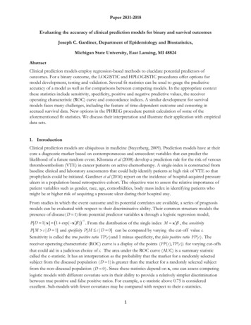
Paper 2831-2018Apply the formats:proc format;value trt 0 'Control' 1 'Treated';value sex 0 'Male' 1 'Female';value affirm 0 'no' 1 'yes';run;proc phreg data survival ph plots rocrocoptions(method ipcw at 6 to 24 by 6 outroc rocdata);class trt (ref 'Control') sex(ref 'Male')diabetic(ref 'no')/param ref;model ITTtime*ITTdeath(0) Trt Age Sex Diabetic Albumin0 nPNA0 GFR0;format trt trt. sex sex. diabetic affirm.;output out stats ph xbeta xbeta;run;The data set STATS PH has the values of the marker XBETA. The marker is practically continuouswith no tied values. Cut-offs c for construction of the ROC are from this support set. Summary statisticsfor XBETA areAnalysis Variable : xbeta Linear PredictorNMean Std Dev Median 25th Pctl 75th Pctl Minimum Maximum256 –1.88741.1337 –1.7475–2.5544–1.0783–5.68301.0384From the formula (3), ROCDATA saves the computation of the estimates of sensitivity ( Sensitivity ( c , t ) ) and specificity ( Specificity 1 FP ( c , t ) ) at the distinct marker values ( Cutoff ). BecauseTPof the request (at 6 to 24 by 6) we have 4 sets of calculations for each of the requested times t.ROCDATA has 1024 256 4 records. The name ITTtime is applied to t. Although default ROC curves,ROC(t) are produced by the plots roc request, the data set ROCDATA has the requisiteinformation for customized plotting. Points on the ROC curve are in descending order of the cutoffvalues going from left to right. If interested in calculating the estimate of AUC(t) from ROCDATA, wemust add to the calculation the area of the trapezoid at the extreme right, that is ( c , t ))(1 TP ( c , t )) where c is the minimum marker value.½(1 FPminminminFigure 1 is obtained from the plot request plots(overlay individual) roc(tick).For each t, the estimated ROC curve ROC(t) is a step function. Sensitivity values change at event times.Estimation of AUC (t)Although ROCDATA has the information to compute the estimate of AUC (t) at the requested timepoints, it is far simpler to apply the options in PHREG statement: our PHM is the same.proc phreg data survival ph plots auc rocoptions(method ipcw iaucoutauc aucdata);5
Paper 2831-2018Figure 1: ROC(t) plots at t 6, 12, 18 and 24 months from the IPCW methodNote that the AT option should not be used when OUTAUC is requested. Estimates of AUC (t)( AUC ) are computed at all event times (79 distinct times for 84 events) and saved in AUCDATA.Summary statistics are:Analysis Variable : AUC Area Under the CurveN Mean Std Dev Median 25th Pctl 75th Pctl Minimum Maximum79 0.78130.03250.78300.76800.78930.64620.996The calculation is simply the sum of the trapezoidal areas under ROC(t). Formula (4) is not needed. Adefault plot is produced by the plots auc request, or use AUCDATA to create a custom plot.6
Paper 2831-2018Figure 2 and the previous table show that AUC(t) is approximately constant at the median 0.7830(shown as a reference line) for times from 6 to 18 months.Figure 2: Estimates of AUC (t) at all event times from the IPCW methodA summary statistic E ( AUC ( T )) is called the integrated (time-dependent) area under the curve (IAUC). It isestimated by a weighted sum of AUC ( t ) with weights w ( t ) Sˆ ( t ) Sˆ ( t ) from the KM estimator ofTTthe event time distribution. The option iauc does the computation as a sum t AUC ( t )w ( t ) over thedistinct event times. The estimate is 0.7795. The range of integration can be restricted to (0, τ) by theTAU option.Confidence intervals AUCThe IPCW method computes standard errors of the estimates of AUC(t) by a sophisticatedperturbation-resampling method. Let {ψ i : 1 i n} be independent and identically distributed (IID)exponential variates with mean 1. Modify formulae (3) as: (c , t ) TPn[ Ti t , M i c ]δ iψ i / SC ( Ti )i 1 n[ Ti t ]δ iψ i / SC ( Ti )and ( c , t ) FPi 1n[ Ti t , M i c ]ψ ii 1 n[ Ti t ]ψ ii 1where M i x′i β , β and SC (.) are modified versions of β̂ and SˆC (.). See PHREG documentation fordetails. We get the standard error σˆ ( t ) of AUC ( t ) based on a specified number (ITER ) of perturbed7
Paper 2831-2018samples and subsequently a 100(1 α)% confidence interval for AUC ( t ) computed asAUC ( t ) z( 1 ½α)σˆ ( t ), AUC ( t ) z 1 ½α σˆ ( t ) . Here z 1 ½α denotes the 100(1 ½α)-th percentile of thestandard normal distribution. The following options save the calculation and produce a plot with the95% confidence limits (pointwise). The defaults are ALPHA .05 and ITER 50.proc phreg data survival ph plots auc rocoptions(method ipcw(cliter 100 seed 13118) outauc aucdata);The plots auc request generates an AUC plot similar to Figure 3 which is recreated from theAUCDATA set.proc sgplot data aucdata noautolegend;series x ITTtime y AUC /lineattrs (thickness 2);band x ITTtime lower lowerAUC upper upperAUC /transparency .5;xaxis values (0 to 28 by 4) label 'ITTtime (months)'labelattrs (weight bold);yaxis labelattrs (weight bold);inset "Based on 100 perturbed samples, IPCW method"/position bottomright;run;Figure 3: Estimates of AUC (t) with 95% confidence intervals at all event times8
Paper 2831-2018Comparison of proportional hazards modelsOur previous discussion employed a PHM with 7 covariates (predictors). Adjusted hazard ratios and95% Wald confidence intervals are obtained via HAZARDRATIO statements (not shown) andcorresponding p-values from Type3 Wald tests. For example, a 0.25-unit increase in baseline albumin isassociated with a reduction in the risk of death by 29%, HR 0.71, 95% CI: 0.60, 0.84. Using theASSESS statement, supremum tests for the functional form of the continuous covariates, and tests ofthe proportional hazards assumption on all covariates indicted no substantive violations of assumptions.Table 1: Hazard ratios and 95% confidence intervals from the PHMDescriptionHazard95%95% p-valueRatio Lower CL Upper CLTRT, Treated vs Control0.6900.4431.075.1013SEX, Female vs Male1.1910.7501.892.4588DIABETIC, yes vs no2.0391.1403.647.0163AGE, Unit 101.2961.0131.660.0394ALBUMIN0, Unit 0.50.7080.5950.843.0001nPNA0, Unit 0.250.6080.4590.807.0006GFR0, Unit 21.0920.9211.294.3111Consider a PHM with the predictors diabetic age Albumin0 nPNA0 GFR0. Call it our Full Model.Now consider sub-models with one or more predictors removed. Multiple ROC statements allow thefitting of the sub-models, a simple comparison of AUC differences and a graphic displaying all the ROCcurves. The format for diabetic is not applied, due to a glitch in the software version used here.proc phreg data survival ph plots(overlay individual) roc(tick)rocoptions(method ipcw(cl iter 50 seed 20918) at 12 aucdiff);model ITTtime*ITTdeath(0) diabetic age Albumin0 nPNA0 GFR0/roclabel 'Full Model';roc "diabetic age Albumin0 nPNA0" diabetic age Albumin0 nPNA0;roc "diabetic age Albumin0" diabetic age Albumin0;roc "diabetic Albumin0 nPNA0" diabetic Albumin0 nPNA0;roc "diabetic Albumin0 nPNA0 GFR0" diabetic Albumin0 nPNA0 GFR0;run;A busy Figure 4 shows ROC curves at t 12 for the 5 models. The plot options were used to insertthe AUC values into the plot. The option aucdiff generates a table of differences in AUC foreach pair of models. Models receive a label from their respective roc statement, and the label for thefull model is supplied in the model statement via ROCLABEL. To suppress comparisons with thefull model use the NOFIT option. Amongst comparisons to the Full model, a 4-variable sub-modelwithout GFR0 would be sufficient. We noticed in Table 1 that GFR0 was not a significant predictor.This sub-model also has the highest AUC and does well in comparison with the other three submodels. However, when a 95% CI for each AUC difference is computed by the UNO method(Table 2), we find that none are significant because the 95% CI straddles the zero value. Figure 4says just about the same.9
Paper 2831-2018Figure 4: ROC curves at t 12 months for Full and Sub-models (IPCW method)Table 2: Estimate at t 12 of AUC difference and 95% confidence limits for model pairsPairID Pair1 diabetic age Albumin0 nPNA0 - diabetic age Albumin02 diabetic age Albumin0 nPNA0 - diabetic Albumin0 nPNA03 diabetic age Albumin0 nPNA0 - diabetic Albumin0 nPNA0GFR04 diabetic age Albumin0 nPNA0 - Full Model5 diabetic age Albumin0 - diabetic Albumin0 nPNA06 diabetic age Albumin0 - diabetic Albumin0 nPNA0 GFR07 diabetic age Albumin0 - Full Model8 diabetic Albumin0 nPNA0 - diabetic Albumin0 nPNA0GFR09 diabetic Albumin0 nPNA0 - Full Model10 diabetic Albumin0 nPNA0 GFR0 - Full Model10AUCLowerUpperEstimate 95% CL 95% CL0.0147 –0.02790.05720.0158 –0.05070.08240.0264 –0.07070.05790.0319
Paper 2831-2018ROC analysis with marker data from an external source ( c , t ) and FP ( c , t ) we need only information on survival dataAs seen in formulae (3) for TP{( Ti , δ i ) : 1 i n} and the marker { M i : 1 i n} . The latter can be generated from another source, forexample an accelerated failure time (AFT) model fitted in LIFEREG or a scale parameter model fitted inSEVERITY. The AFT is a parametric model with the form log( T ) x′β σε where ε has a specifiedparametric distribution. When ε has the logistic distribution we get the log-logistic survival distribution(1 {t / θ ( x )} ) ; when ε has the extreme-value distribution we get the Weibull survival x ) exp (( t / θ ( x )) σ ) where σ 0 is a shape parameter and log θ ( x ) x′β (Gardinerdistribution S ( t 1/σS ( t x ) 11/et al, 2014). The Weibull has the proportional hazards property but the log-logistic does not. In AFTmodels a higher value of the marker M x′β is indicative of better survival. Therefore, we must flip thesign of the marker to keep in line with our previous discussion of the Cox PHM.The following syntax fits the log-logistic model with all 7 covariates. Change the DIST option todist Weibull to fit the Weibull.proc lifereg data survival ph;class trt sex diabetic;format trt trt. sex sex. diabetic affirm.;model ITTtime*ITTdeath(0) Trt Age Sex Diabetic Albumin0 nPNA0GFR0/dist llogistic;output out stats lr xbeta xbeta l;run;The Weibull shows close similarity with our previous PHM (Table 3).Table 3: Type III Analysis of 111111LOG-LOGISTICMODELWald 6454.84990.027616.5919 .00019.41320.00220.27500.6000WEIBULL 0.00080.3190Cox PH 0.00060.3111Create the marker data for log-logistic and Weibull models in the same data set. This may be done by (1)fit log-logistic and save XBETA l, (2) use the output file to fit Weibull and save XBETA w, (3) flip signto get marker l and marker w in the data set stats lr3. The now familiar syntax produces the ROCcurves at two time points for the three models (Figure 5).11
Paper 2831-2018proc phreg data stats lr3 plots(overlay individual) roc(tick)rocoptions(method ipcw at 12,18);class trt (ref 'Control') sex(ref 'Male') diabetic(ref 'no')/param ref;format trt trt. sex sex. diabetic affirm.;model ITTtime*ITTdeath(0) Trt Age Sex Diabetic Albumin0 nPNA0GFR0/roclabel 'Proportional Hazards Model';roc "Log-logistic Model" pred marker l;roc "Weibull Model" pred marker w;run;Figure 5: ROC curves at t 12, 18 months for Log-logistic, Weibull and Cox PH modelsChecking independence of the censoring distribution and markerThe IPCW method assumes that the censoring distribution is not dependent on the marker M. Aninformal check of this assumption can be made by plotting the KM estimates SˆC ( t ) in strata defined bythe values of M. First, fit a PHM and save the marker data. Second, create categories for thedistribution of M. We use tertiles to create 3 strata. Third, obtain KM estimates from LIFETEST with aSTRATA statement.The PHM fitted isproc phreg data survival ph;class diabetic(ref 'no')/param ref;model ITTtime*ITTdeath(0) Diabetic Age Albumin0 nPNA0;format diabetic affirm.;output out stats ph xbeta xbeta;run;12
Paper 2831-2018Tertiles of the marker are obtained from UNIVARIATE:proc univariate data stats ph;var xbeta;output out xb pctl pctlpts ( 33 66) pctlpre P ;run;Issue a format to create 3 tertiles categories T1, T2, T3:proc format;value trtl low- -2.26350 'T1' -2.26350- -1.23428 'T2'-1.23428-high 'T3';run;Obtain KM estimates for the event time distribution and separately for the censoring time distribution:ods output survivalplot surv T; /*surv C*/proc lifetest data stats phplots survival(atrisk (0 to 30 by 6) atrisktickonly nocensortest);strata xbeta/test logrank;format xbeta trtl.;time ITTtime*ITTdeath(0); *ITTtime*ITTdeath(1);label ITTtime 'ITTtime (months)';run;For purposes of plotting, two ODS output data sets are created. Two invocations of SGPLOT willcreate an enhanced plot of the event time distribution and censoring distribution (Matange, 2016). Thesyntax for the latter is:ods graphics on/height 4.2in width 3.2in;proc sgplot data surv C noautolegend;step x time y survival /group stratum lineattrs (thickness 1);xaxistable atrisk/x tatrisk class stratum location insidecolorgroup stratum valueattrs (size 9)title " Atrisk by Tertiles of Marker";xaxis values (0 to 30 by 6) labelattrs (weight bold);yaxis label "Survival Probability (Censoring)"labelattrs (weight bold);inset "Logrank p .2858" / border textattrs (size 9) position s;run;The plots are in Figure 6. To show detail, the vertical scale is different for the two plots. We expect asignificant association of the marker with the event time (left panel), and fortunately we find noassociation of the marker with the censoring time (right panel)—at least from the informal investigationmade here. Assessments are based on the log-rank test.13
Paper 2831-2018Figure 6: KM estimates of event time and censoring distributions by marker categoriesWhen the censoring distribution is dependent on the marker, some arguments of the IPCW method forconsistency of estimators break down. Blanche et al (2013a) offer a modification of the IPCW methodcalled the conditional IPCW (CIPCW) which replaces the observation weights in formulae (3) for ( c , t ) by δ Sˆ ( T M ) 1 and introduces a weight Sˆ ( t M ) 1 in FP ( c , t ) . They suggest a CoxTPi{Cii{}Ci}PMH or any other model be applied to estimate SC ( t M ) or preferably from the bivariate distributionP[C t , M c ] . Via simulation studies, the CIPCW estimators show robustness to dependency of thecensoring distribution on the marker and perform well in comparison to the nearest neighbor methodwhich is the default method in PHREG.Nearest Neighbor Method (METHOD NNE)PHREG offers METHOD NNE for the nearest neighbor approach (Heagerty et al, 2000) based on abivariate survival distribution for (M, T) introduced by Akritas (1994). The NNE method is not currentlyfully developed: we can get the relevant estimates for ROC analysis, but standard errors are not availablefor the estimator of AUC ( t ) . Consistency and asymptotic normality have been established, but thedifficulty lies in estimating the asymptotic variance. Resampling methods could be used (Hung andChiang, 2010a, 2011).14
Paper 2831-2018Using the data {( Ti , δ i , x i ) : 1 i n} with the marker M i x′i βˆ , estimate the bivariate survivalnSˆbn ( c , t ) n 1 i 1 Sˆ M i )[ M i c ] . The conditionaldistribution of S ( c , t ) P[ M c , T t ] by bn ( t Msurvival distribution is estimated by a kernel-smoothed weighted KM-estimator, Sˆbn ( t M Mi ) j K bn ( M i , M j )[ T j* s ]δ j 1 s t j K bn ( M i , M j )[T j* s ] , M j ) [ FM ( M i ) FM ( M j ) bn ], 0 bn ½ and FM (.) is the cumulative distributionwhere K ( M i function (CDF) of the marker M. Ties amongst observed times are allowed (just as in KM). At themarker value M i , j K bn ( M i , M j )[ T j* s ]δ j counts events at time T j* s whose associated markervalue M j is to close M i ; also jK bn ( M i , M j )[ T j* s ] is the risk set at time s, but restricted toindividuals whose maker value is close to M i . By default bandwidth bn 0.05, so that 10% of nearestneighbors are used. Use option SPAN to change setting. A suggested choice is bn O( n 1/3 ) .True Positive Ratio (Sensitivity )and False Positive Ratio (1 Specificity)Directly from their definitions we get the corresponding estimators FM ( c ) Sˆbb ( c , t ) Sˆbb ( c , t ) ( c , t ) 1 ., FP ( c , t )TP1 Sˆbn ( , t )Sˆbn ( , t )These estimators are monotone in c and bounded on [0.1].Consider the same models described in the previous section for the log-logistic, Weibull, and CoxPHM with covariates Trt Age Sex Diabetic Albumin0 nPNA0 GFR0. ROC analysisusing the NNE method requires only one change in the rocoptions.proc phreg data stats lr3 plots(overlay individual) roc(tick)rocoptions(method NNE at 12, 18 outroc rocdata);class trt (ref 'Control') sex(ref 'Male')diabetic(ref 'no')/param ref;format trt trt. sex sex. diabetic affirm.;model ITTtime*ITTdeath(0) Trt Age Sex Diabetic Albumin0 nPNA0GFR0/roclabel 'Proportional Hazards Model';roc "Log-logistic Model" pred marker l;roc "Weibull Model" pred marker w;run;Figure 7 plots the ROC curves. Notice that the NNE method produces smoother curves than the IPCWmethod. The AUC can be computed by the trapezoidal rule from the output data set ROCDATA.15
Paper 2831-2018Figure 7: ROC curves at t 12, 18 by the NNE methodRecursive Method (METHOD RECURSIVE)This method proposed by Chambless and Diao (2006) for estimation of TP ( c , t ), FP ( c , t ), AUC ( t )follows a recursive computation using the ordered distinct survival times up to t. Explicit formulae areavailable for the three estimators. Unfortunately, the estimator of FP ( c , t ) need not be monotone in c orbounded in [0,1]. The
Clinical prediction models employ regression-based methods to elucidate potential predictors of outcomes. For a binary outcome, the LOGISTIC and HPLOGISTIC procedures offer options for