Transcription
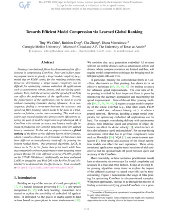
Towards Efficient Model Compression via Learned Global RankingTing-Wu Chin1 , Ruizhou Ding1 , Cha Zhang2 , Diana Marculescu13Carnegie Mellon University1 , Microsoft Cloud and AI2 , The University of Texas at Austin3{tingwuc, rding}@andrew.cmu.edu, chazhang@mirosoft.com, dianam@utexas.eduAbstractPruning convolutional filters has demonstrated its effectiveness in compressing ConvNets. Prior art in filter pruning requires users to specify a target model complexity (e.g.,model size or FLOP count) for the resulting architecture.However, determining a target model complexity can bedifficult for optimizing various embodied AI applicationssuch as autonomous robots, drones, and user-facing applications. First, both the accuracy and the speed of ConvNetscan affect the performance of the application. Second,the performance of the application can be hard to assesswithout evaluating ConvNets during inference. As a consequence, finding a sweet-spot between the accuracy andspeed via filter pruning, which needs to be done in a trialand-error fashion, can be time-consuming. This work takesa first step toward making this process more efficient by altering the goal of model compression to producing a set ofConvNets with various accuracy and latency trade-offs instead of producing one ConvNet targeting some pre-definedlatency constraint. To this end, we propose to learn a globalranking of the filters across different layers of the ConvNet,which is used to obtain a set of ConvNet architectures thathave different accuracy/latency trade-offs by pruning thebottom-ranked filters. Our proposed algorithm, LeGR, isshown to be 2 to 3 faster than prior work while having comparable or better performance when targeting sevenpruned ResNet-56 with different accuracy/FLOPs profileson the CIFAR-100 dataset. Additionally, we have evaluatedLeGR on ImageNet and Bird-200 with ResNet-50 and MobileNetV2 to demonstrate its effectiveness. Code availableat https://github.com/cmu-enyac/LeGR.1. IntroductionBuilding on top of the success of visual perception [49,17, 18], natural language processing [10, 11], and speechrecognition [6, 45] with deep learning, researchers havestarted to explore the possibility of embodied AI applications. In embodied AI, the goal is to enable agents to takeactions based on perceptions in some environments [51].We envision that next generation embodied AI systemswill run on mobile devices such as autonomous robots anddrones, where compute resources are limited and thus, willrequire model compression techniques for bringing such intelligent agents into our lives.In particular, pruning the convolutional filters in ConvNets, also known as filter pruning, has shown to be aneffective technique [63, 36, 60, 32] for trading accuracyfor inference speed improvements. The core idea of filter pruning is to find the least important filters to prune byminimizing the accuracy degradation and maximizing thespeed improvement. State-of-the-art filter pruning methods [16, 20, 36, 70, 46, 8] require a target model complexity of the whole ConvNet (e.g., total filter count, FLOPcount1 , model size, inference latency, etc.) to obtain apruned network. However, deciding a target model complexity for optimizing embodied AI applications can behard. For example, considering delivery with autonomousdrones, both inference speed and precision of object detectors can affect the drone velocity [3], which in turn affects the inference speed and precision2 . For an user-facingautonomous robot that has to perform complicated taskssuch as MovieQA [56], VQA [2], and room-to-room navigation [1], both speed and accuracy of the visual perception module can affect the user experience. These aforementioned applications require many iterations of trial-anderror to find the optimal trade-off point between speed andaccuracy of the ConvNets.More concretely, in these scenarios, practitioners wouldhave to determine the sweet-spot for model complexity andaccuracy in a trial-and-error fashion. Using an existing filter pruning algorithm many times to explore the impactof the different accuracy-vs.-speed trade-offs can be timeconsuming. Figure 1 demonstrates the usage of filter pruning for optimizing ConvNets in aforementioned scenarios.With prior approaches, one has to go through the process offinding constraint-satisfying pruned-ConvNets via a prun1 The number of floating-point operations to be computed for a ConvNetto carry out an inference.2 Higher velocity requires faster computation and might cause accuracydegradation due to the blurring effect of the input video stream.11518
2. Related WorkVarious methods have been developed to compressand/or accelerate ConvNets including weight quantization [47, 71, 29, 30, 65, 24, 12, 7], efficient convolution operators [25, 22, 61, 26, 67], neural architecture search [69,9, 4, 15, 54, 53, 52], adjusting image resolution [55, 5],and filter pruning, considered in this paper. Prior art on filter pruning can be grouped into two classes, depending onwhether the architecture of the pruned-ConvNet is assumedto be given.Figure 1: Using filter pruning to optimize ConvNets for embodied AI applications. Instead of producing one ConvNetfor each pruning procedure as in prior art, our proposedmethod produces a set of ConvNets for practitioners to efficiently explore the trade-offs.ing algorithm for every model complexity considered until practitioners are satisfied with the accuracy-vs.-speeduptrade-off. Our work takes a first step toward alleviating theinefficiency in the aforementioned paradigm. We propose toalter the objective of pruning from outputting a single ConvNet with pre-defined model complexity to producing a setof ConvNets that have different accuracy/speed trade-offs,while achieving comparable accuracy with state-of-the-artmethods (as shown in Figure 4). In this fashion, the modelcompression overhead can be greatly reduced, which resultsin a more practical usage of filter pruning.To this end, we propose learned global ranking (orLeGR), an algorithm that learns to rank convolutional filters across layers such that the ConvNet architectures ofdifferent speed/accuracy trade-offs can be obtained easilyby dropping the bottom-ranked filters. The obtained architectures are then fine-tuned to generate the final models. Insuch a formulation, one can obtain a set of architectures bylearning the ranking once. We demonstrate the effectivenessof the proposed method with extensive empirical analysesusing ResNet and MobileNetV2 on CIFAR-10/100, Bird200, and ImageNet datasets. The main contributions of thiswork are as follows: We propose learned global ranking (LeGR), which produces a set of pruned ConvNets with different accuracy/speed trade-offs. LeGR is shown to be faster thanprior art in ConvNet pruning, while achieving comparable accuracy with state-of-the-art methods on threedatasets and two types of ConvNets. Our formulation towards pruning is the first work thatconsiders learning to rank filters across different layersglobally, which addresses the limitation of prior art inmagnitude-based filter pruning.Pre-defined architecture In this category, various workproposes different metrics to evaluate the importance of filters locally within each layer. For example, some priorwork [32, 19] proposes to use 2 -norm of filter weights asthe importance measure. On the other hand, other workhas also investigated using the output discrepancy betweenthe pruned and unpruned network as an importance measure [23, 40]. However, the key drawback for methods thatrank filters locally within a layer is that it is often hard todecide the overall target pruned architectures [20]. To copewith this difficulty, uniformly pruning the same portion offilters across all the layers is often adopted [19].Learned architecture In this category, pruning algorithms learn the resulting structure automatically given acontrollable parameter to determine the complexity of thepruned-ConvNet. To encourage weights with small magnitudes, Wen et al. [60] propose to add group-Lasso regularization to the filter norm to encourage filter weights to bezeros. Later, Liu et al. [36] propose to add Lasso regularization on the batch normalization layer to achieve pruningduring training. Gordon et al. [16] propose to add computeweighted Lasso regularization on the filter norm. Huanget al. [27] propose to add Lasso regularization on the output neurons instead of weights. While the regularizationpushes unimportant filters to have smaller weights, the final thresholding applied globally assumes different layersto be equally important. Later, Louizos et al. [39] have proposed L0 regularization with stochastic relaxation. From aBayesian perspective, Louizos et al. [38] formulate pruning in a probabilistic fashion with a sparsity-induced prior.Similarly, Zhou et al. [70] propose to model inter-layer dependency. From a different perspective, He et al. proposean automated model compression framework (AMC) [20],which uses reinforcement learning to search for a ConvNetthat satisfies user-specified complexity constraints.While these prior approaches provide competitivepruned-ConvNets under a given target model complexity,it is often hard for one to specify the complexity parameterwhen compressing a ConvNet in embodied AI applications.To cope with this, our work proposes to generate a set of1519
pruned-ConvNets across different complexity values ratherthan a single pruned-ConvNet under a target model complexity.We note that some prior work gradually prunes the ConvNet by alternating between pruning out a filter and finetuning, and thus, can also obtain a set of pruned-ConvNetswith different complexities. For example, Molchanov etal. [43] propose to use the normalized Taylor approximation of the loss as a measure to prune filters. Specifically,they greedily prune one filter at a time and fine-tune the network for a few gradient steps before the pruning proceeds.Following this paradigm, Theis et al. [57] propose to switchfrom first-order Taylor to Fisher information. However, ourexperiment results show that the pruned-ConvNet obtainedby these methods have inferior accuracy compared to themethods that generate a single pruned ConvNet.To obtain a set of ConvNets across different complexities with competitive performance, we propose to learn aglobal ranking of filters across different layers in a datadriven fashion such that architectures with different complexities can be obtained by pruning out the bottom-rankedfilters.3. Learned Global RankingThe core idea of the proposed method is to learn a ranking for filters across different layers such that a ConvNet ofa given complexity can be obtained easily by pruning outthe bottom rank filters. In this section, we discuss our assumptions and formulation toward achieving this goal.As mentioned earlier in Section 1, often both accuracyand latency of a ConvNet affect the performance of the overall application. The goal for model compression in thesesettings is to explore the accuracy-vs.-speed trade-off forfinding a sweet-spot for a particular application using modelcompression. Thus, in this work, we use FLOP count for themodel complexity to sample ConvNets. As we will show inSection 5.3, we find FLOP count to be predictive for latency.3.1. Global RankingTo obtain pruned-ConvNets with different FLOP counts,we propose to learn the filter ranking globally across layers. In such a formulation, the global ranking for a givenConvNet just needs to be learned once and can be usedto obtain ConvNets with different FLOP counts. However, there are two challenges for such a formulation. First,the global ranking formulation enforces an assumption thatthe top-performing smaller ConvNets are a proper subsetof the top-performing larger ConvNets. The assumptionmight be strong because there are many ways to set the filter counts across different layers to achieve a given FLOPcount, which implies that there are opportunities where thetop-performing smaller network can have more filter countsin some layers but fewer filter counts in some other layerscompared to a top-performing larger ConvNet. Nonetheless, this assumption enables the idea of global filter ranking, which can generate pruned ConvNets with differentFLOP counts efficiently. In addition, the experiment resultsin Section 5.1 show that the pruned ConvNets under thisassumption are competitive in terms of performance withthe pruned ConvNets obtained without this assumption. Westate the subset assumption more formally below.Assumption 1 (Subset Assumption) For an optimalpruned ConvNet with FLOP count f , let F(f )l be thefilter count for layer l. The subset assumption states thatF(f )l F(f 0 )l 8 l if f f 0 .Another challenge for learning a global ranking is thehardness of the problem. Obtaining an optimal global ranking can be expensive, i.e., it requires O(K K!) rounds ofnetwork fine-tuning, where K is the number of filters. Thus,to make it tractable, we assume the filter norm is able torank filters locally (intra-layer-wise) but not globally (interlayer-wise).Assumption 2 (Norm Assumption) 2 norm can be usedto compare the importance of a filter within each layer, butnot across layers.We note that the norm assumption is adopted and empirically verified by prior art [32, 62, 20]. For filter norms tobe compared across layers, we propose to learn layer-wiseaffine transformations over filter norms. Specifically, theimportance of filter i is defined as follows:2Ii l(i) kΘi k2 l(i) ,(1)where l(i) is the layer index for the ith filter, k·k2 denotes 2 norms, Θi denotes the weights for the ith filter, and α 2RL , κ 2 RL are learnable parameters that represent layerwise scale and shift values, and L denotes the number oflayers. We will detail in Section 3.2 how α-κ pairs arelearned so as to maximize overall accuracy.Based on these learned affine transformations fromEq. (1) (i.e., the α-κ pair), the LeGR-based pruning proceeds by ranking filters globally using I and prunes awaybottom-ranked filters, i.e., smaller in I, such that the FLOPcount of interest is met, as shown in Figure 2. This process can be done efficiently without the need of trainingdata (since the knowledge of pruning is encoded in the α-κpair).3.2. Learning Global RankingTo learn α and κ, one can consider constructing a ranking with α and κ and then uniformly sampling ConvNetsacross different FLOP counts to evaluate the ranking. However, ConvNets obtained with different FLOP counts havedrastically different validation accuracy, and one has to1520
2Figure 2: The flow of LeGR-Pruning. kΘk2 represents the filter norm. Given the learned layer-wise affine transformations,i.e., the α-κ pair, LeGR-Pruning returns filter masks that determine which filters are pruned. After LeGR-Pruning, the prunednetwork will be fine-tuned to obtain the final network.know the Pareto curve3 of pruning to normalize the validation accuracy across ConvNets obtained with differentFLOP counts. To address this difficulty, we propose to evaluate the validation accuracy of the ConvNet obtained fromthe lowest considered FLOP count as the objective for theranking induced by the α-κ pair. Concretely, to learn α andκ, we treat LeGR as an optimization problem:arg max Accval (Θ̂l )(2)Θ̂l LeGR-Pruning(α, κ, ˆl ).(3)Algorithm 1 Learning α, κ with regularized EAInput: model Θ, lowest constraint ˆl , random walk size, total search iterations E, sample size S, mutation ratiou, population size P , fine-tune iterations ˆOutput: α, κInitialize P ool to a size P queuefor e 1 to E doα 1, κ 0if P ool has S samples thenV P ool.sample(S)α, κ argmaxFitness(V )end ifLayer Sample u% layers to mutatefor l 2 Layer dostdl computeStd([Mi 8 i 2 l])2αl αl α̂l , where α̂l eN (0,σ )κl κl κ̂l , where κ̂l N (0,stdl )end forΘ̂l LeGR-Pruning-and-fine-tuning(α, κ, ˆl , ˆ, Θ)F itness Accval (Θ̂l )P ool.replaceOldestWith(α, κ, F itness)end forα,κwhereLeGR-Pruning prunes away the bottom-ranked filters untilthe desired FLOP count is met as shown in Figure 2. ˆldenotes the lowest FLOP count considered. As we will discuss later in Section 5.1, we have also studied how ˆ affectsthe performance of the learned ranking, i.e., how the learnedranking affects the accuracy of the pruned networks.Specifically, to learn the α-κ pair, we rely on approachesfrom hyper-parameter optimization literature. While thereare several options for the optimization algorithm, weadopt the regularized evolutionary algorithm (EA) proposedin [48] for its effectiveness in the neural architecture searchspace. The pseudo-code for our EA is outlined in Algorithm 1. We have also investigated policy gradients for solving for the α-κ pair, which is shown in Appendix B. We canequate each α-κ pair to a network architecture obtained byLeGR-Pruning. Once a pruned architecture is obtained, wefine-tune the resulting architecture by ˆ gradient steps anduse its accuracy on the validation set4 as the fitness (i.e.,3 A Pareto curve describes the optimal trade-off curve between two metrics of interest. Specifically, one cannot obtain improvement in one metricwithout degrading the other metric. The two metrics we considered in thiswork are accuracy and FLOP count.4 We split 10% of the original training set to be used as validation set.validation accuracy) for the corresponding α-κ pair. Wenote that we use ˆ to approximate (fully fine-tuned steps)and we empirically find that ˆ 200 gradient updates workwell under the pruning settings across the datasets and networks we study. More concretely, we first generate a pool ofcandidates (α and κ values) and record the fitness for eachcandidate, and then repeat the following steps: (i) sample asubset from the candidates, (ii) identify the fittest candidate,(iii) generate a new candidate by mutating the fittest candidate and measure its fitness accordingly, and (iv) replace theoldest candidate in the pool with the generated one. To mu1521
tate the fittest candidate, we randomly select a subset of thelayers Layer and conduct one step of random-walk fromtheir current values, i.e., l , l 8 l 2 Layer.We note that our layer-wise affine transformation formulation (Eq. 1) can be interpreted from an optimizationperspective. That is, one can upper-bound the loss difference between a pre-trained ConvNet and its pruned-andfine-tuned counterpart by assuming Lipschitz continuity onthe loss function, as detailed in Appendix A.4. Evaluations4.1. Datasets and Training SettingOur work is evaluated on various image classificationbenchmarks including CIFAR-10/100 [31], ImageNet [50],and Birds-200 [58]. CIFAR-10/100 consists of 50k trainingimages and 10k testing images with a total of 10/100 classesto be classified. ImageNet is a large scale image classification dataset that includes 1.2 million training images and50k testing images with 1k classes to be classified. Also,we benchmark the proposed algorithm in a transfer learningsetting since in practice, we want a small and fast modelon some target datasets. Specifically, we use the Birds-200dataset that consists of 6k training images and 5.7k testingimages covering 200 bird species.For Bird-200, we use 10% of the training data as the validation set used for early stopping and to avoid over-fitting.The training scheme for CIFAR-10/100 follows [19], whichuses stochastic gradient descent with nesterov [44], weightdecay 5e 4 , batch size 128, 1e 1 initial learning rate withdecrease by 5 at epochs 60, 120, and 160, and train for200 epochs in total. For control experiments with CIFAR100 and Bird-200, the fine-tuning after pruning is done asfollows: we keep all training hyper-parameters the samebut change the initial learning rate to 1e 2 and train for 60epochs (i.e., 21k). We drop the learning rate by 10 at30%, 60%, and 80% of the total epochs, i.e., epochs 18, 36,and 48. To compare numbers with prior art on CIFAR-10and ImageNet, we follow the number of iterations in [72].Specifically, for CIFAR-10 we fine-tuned for 400 epochswith initial learning rate 1e 2 , drop by 5 at epochs 120,240, and 320. For ImageNet, we use pre-trained models andwe fine-tuned the pruned models for 60 epochs with initiallearning rate 1e 2 , drop by 10 at epochs 30 and 45.For the hyper-parameters of LeGR, we select ˆ 200,i.e., fine-tune for 200 gradient steps before measuring thevalidation accuracy when searching for the α-κ pair. Wenote that we do the same for AMC [20] for a fair comparison. Moreover, we set the number of architectures exploredto be the same with AMC, i.e., 400. We set mutation rateu 10 and the hyper-parameter of the regularized evolutionary algorithm by following prior art [48]. In the following experiments, we use the smallest considered as ˆlto search for the learnable variables α and κ. The foundα-κ pair is used to obtain the pruned networks at variousFLOP counts. For example, for ResNet-56 with CIFAR100 (Figure 3a), we use ˆl 20% to obtain the α-κ pairand use the same α-κ pair to obtain the seven networks( 20%, ., 80%) with the flow described in Figure 2.The ablation of ˆl and ˆ are detailed in Sec. 5.2.We prune filters across all the convolutional layers. Wegroup dependent channels by summing up their importancemeasure and prune them jointly. The importance measurerefers to the measure after learned affine transformations.Specifically, we group a channel in depth-wise convolution with its corresponding channel in the preceding layer.We also group channels that are summed together throughresidual connections.4.2. CIFAR-100 ResultsIn this section, we consider ResNet-56 and MobileNetV2 and we compare LeGR mainly with four filterpruning methods, i.e., MorphNet [16], AMC [20], FisherPruning [57], and a baseline that prunes filters uniformlyacross layers. Specifically, the baselines are determinedsuch that one dominant approach is selected from different groups of prior art. We select one approach [16]from pruning-while-learning approaches, one approach [20]from pruning-by-searching methods, one approach [57]from continuous pruning methods, and a baseline extendingmagnitude-based pruning to various FLOP counts. We notethat FisherPruning is a continuous pruning method wherewe use 0.0025 learning rate and perform 500 gradient stepsafter each filter pruned following [57].As shown in Figure 3a, we first observe that FisherPruning does not work as well as other methods and we hypothesize the reason for it is that the small fixed learning rate inthe fine-tuning phase makes it hard for the optimizer to getout of local optima. Additionally, we find that FisherPruning prunes away almost all the filters for some layers. Onthe other hand, we find that all other approaches outperformthe uniform baseline in a high-FLOP-count regime. However, both AMC and MorphNet have higher variances whenpruned more aggressively. In both cases, LeGR outperformsprior art, especially in the low-FLOP-count regime.More importantly, our proposed method aims to alleviatethe cost of pruning when the goal is to explore the trade-offcurve between accuracy and inference latency. From thisperspective, our approach outperforms prior art by a significant margin. More specifically, we measure the averagetime of each algorithm to obtain the seven pruned ResNet56 across the FLOP counts in Figure 3a using our hardware (i.e., NVIDIA GTX 1080 Ti). Figure 3b shows theefficiency of AMC, MorphNet, FisherPruning, and the proposed LeGR. The cost can be broken down into two parts:(1) pruning: the time it takes to search for a network that has1522
(b)(a)Figure 3: (a) The trade-off curve of pruning ResNet-56 and MobileNetV2 on CIFAR-100 using various methods. We averageacross three trials and plot the mean and standard deviation. (b) Training cost for seven ConvNets across FLOP counts usingvarious methods targeting ResNet-56 on CIFAR-100. We report the average cost considering seven FLOP counts, i.e., 20%to 80% FLOP count in a step of 10% on NVIDIA GTX 1080 Ti. The cost is normalized to the cost of LeGR.some pre-defined FLOP count and (2) fine-tuning: the timeit takes for fine-tuning the weights of a pruned network. ForMorphNet, we consider three trials for each FLOP countto find an appropriate hyper-parameter to meet the FLOPcount of interest. The numbers are normalized to the costof LeGR. In terms of pruning time, LeGR is 7 and 5 faster than AMC and MorphNet, respectively. The efficiency comes from the fact that LeGR only searches the ακ pair once and re-uses it across FLOP counts. In contrast,both AMC and MorphNet have to search for networks forevery FLOP count considered. FisherPruning always pruneone filter at a time, and therefore the lowest FLOP countlevel considered determines the pruning time, regardless ofhow many FLOP count levels we are interested in.Table 1: Comparison with prior art on CIFAR-10. We groupmethods into sections according to different FLOP counts.Values for our approaches are averaged across three trialsand we report the mean and standard deviation. We useboldface to denote the best numbers and use to denote ourimplementation. The accuracy is represented in the formatof pre-trained 7! pruned-and-fine-tuned.N ETWORKM ETHODACC . (%)R ES N ET-56PF [32]TAYLOR [43] L E GRDCP-A DAPT [72]CP [23]AMC [20]DCP [72]SFP [19]L E GR93.0 93.093.9 93.293.9 94.1 0.093.8 93.892.8 91.892.8 91.993.8 93.593.6 0.6 93.4 0.393.9 93.7 0.290.9 (72%)90.8 (72%)87.8 (70%)66.3 (53%)62.7 (50%)62.7 (50%)62.7 (50%)59.4 (47%)58.9 (47%)VGG-13BC-GNJ [38]BC-GHS [38]VIBN ET [8]L E GR91.9 91.491.9 9191.9 91.591.9 92.4 0.2141.5 (45%)121.9 (39%)70.6 (22%)70.3 (22%)4.3. Comparison with Prior ArtAlthough the goal of this work is to develop a modelcompression method that produces a set of ConvNets acrossdifferent FLOP counts, we also compare our method withprior art that focuses on generating a ConvNet for a specified FLOP count.CIFAR-10 In Table 1, we compare LeGR with prior artthat reports results on CIFAR-10. First, for ResNet-56, wefind that LeGR outperforms most of the prior art in bothFLOP count and accuracy dimensions and performs similarly to [19, 72]. For VGG-13, LeGR achieves significantlybetter results compared to prior art.ImageNet Results For ImageNet, we prune ResNet-50and MobileNetV2 with LeGR to compare with prior art.For LeGR, we learn the ranking using 47% FLOP countfor ResNet-50 and 50% FLOP count for MobileNetV2, anduse the learned ranking to obtain ConvNets for other FLOPMFLOPCOUNTcounts of interest. We have compared to 17 prior methods that report pruning performance for ResNet-50 and/orMobileNetV2 on the ImageNet dataset. While our focusis on the fast exploration of the speed and accuracy tradeoff curve for filter pruning, our proposed method is betteror comparable compared to the state-of-the-art methods asshown in Figure 4. The detailed numerical results are inAppendix C. We would like to emphasize that to obtaina pruned-ConvNet with prior methods, one has to run thepruning algorithm for every FLOP count considered. Incontrast, our proposed method learns the ranking once anduses it to obtain ConvNets across different FLOP counts.1523
Figure 4: Results for ImageNet. LeGR is better or comparable compared to prior methods. Furthermore, its goal is to outputa set of ConvNets instead of one ConvNet. The detailed numerical results are in Appendix C.4.4. Transfer Learning: Bird-200We analyze how LeGR performs in a transfer learning setting where we have a model pre-trained on a largedataset, i.e., ImageNet, and we want to transfer its knowledge to adapt to a smaller dataset, i.e., Bird-200. We prunethe fine-tuned network on the target dataset directly following the practice in prior art [68, 40]. We first obtain finetuned MobileNetV2 and ResNet-50 on the Bird-200 datasetwith top-1 accuracy 80.2% and 79.5%, respectively. Theseare comparable to the reported values in prior art [33, 41].As shown in Figure 5, we find that LeGR outperforms Uniform and AMC, which is consistent with previous analysesin Section 4.2.Figure 5: Results for Bird-200.5. Ablation Study5.1. Ranking Performance and ˆlTo learn the global ranking with LeGR without knowingthe Pareto curve in advance, we use the minimum consid-Figure 6: Robustness to the hyper-parameter ˆl . Prior art isplotted as a reference (c.f. Figure 3a).ered FLOP count ( ˆl ) during learning to evaluate the performance of a ranking. We are interested in understandinghow this design choice affects the performance of LeGR.Specifically, we try LeGR targeting ResNet-56 for CIFAR100 with ˆl 2 {20%, 40%, 60%, 80%}. As shown in Figure 6, we first observe that rankings learned using different FLOP counts have similar performances, which empirically supports Assumption 1. More concretely, consider thenetwork pruned to 40% FLOP count by using the rankinglearned at 40% FLOP count. This case does not take advantage of the subset assumption because the entire learningprocess for learning α-κ is done only by looking at the performance of the 40% FLOP count network. On the otherhand, rankings learned using other FLOP counts but employed to obtain pruned-networks at 40% FLOP count haveexploited the subset assumption (e.g., the ranking learnedfor 80% FLOP count can produce a competitive network1524
Figure 7: Pruning ResNet-56 for CIFAR-100 with LeGR bylearning α and κ using different ˆ and FLOP count constraints.for 40% FLOP count). We find that LeGR with or withoutemploying Assumption 1 results in similar performance forthe pruned networks.Figure 8: Latency reduction vs. FLOP count reduction.FLOP count reduction is indicative for latency reduction.of size 224x224 and the program (Python with PyTorch) isrun using a single thread. As shown in Figure 8, filter pruning can produce near-linear acceleration (with a slope of approximately 0.6) without specialized software or hardwaresupport.5.2. Fine-tuned IterationsSinc
effective technique [63, 36, 60, 32] for trading accuracy for inference speed improvements. The core idea of fil-ter pruning is to find the least important filters to prune by minimizing the accuracy degradation and maximizing the speed improvement. State-of-the-art filter pruning meth-od