Transcription
research methodology seriesAn Introductionto Secondary Data AnalysisNatalie Koziol, MACYFS Statistics and Measurement ConsultantAnn Arthur, MSCYFS Statistics and Measurement Consultant
Outline Overview of Secondary Data AnalysisUnderstanding & Preparing Secondary DataBrief Overview of Sampling DesignAnalyzing Secondary DataIllustration of Secondary Data AnalysisOther Logistical Considerations
Overview ofSecondary Data Analysis
What is Secondary Data Analysis? “In the broadest sense, analysis of data collected by someone else”(p. ix; Boslaugh, 2007) Analysis of secondary data, where “secondary data can include anydata that are examined to answer a research question other than thequestion(s) for which the data were initially collected”(p. 3; Vartanian, 2010) In contrast to primary data analysis in which the same individual/teamof researchers designs, collects, and analyzes the data
Local Examples of Research InvolvingSecondary Data Analysis Starting Off Right: Effects of Rurality on Parent‟s Involvement inChildren‟s Early Learning (Sue Sheridan, PPO)– Data from the Early Childhood Longitudinal Study – Birth Cohort(ECLS-B) were used to examine the influence of setting on parentalinvolvement in preschool and the effects of involvement onKindergarten school readiness. Testing Thresholds of Quality Care on Child Outcomes Globally & inSubgroups: Secondary Analysis of QUINCE and Early Head Start Data(Helen Raikes, PPO)– Data from two secondary datasets were used to examine thepotentially non-linear relationship between quality of child care andchildren‟s development
What are Secondary Data? Come from many sources– Large government-funded datasets (the focus of this presentation)– University/college records– Statewide or district-level K-12 school records– Journal supplements– Authors‟ websites– Etc.! Available for a seemingly unlimited number of subject areas Quantitative (the focus of this presentation) and qualitative Restricted and public-use Direct (e.g., biomarker data) and indirect observation (e.g., self-report)
Where Can I Find Secondary Data?Searching for secondary datasets: Inter-University Consortium for Political and Social Research– ndex.jsp Data.gov– http://www.data.gov National Center for Education Statistics– http://nces.ed.gov U.S. Census Bureau– http://www.census.gov Simple Online Data Archive for Population Studies (SodaPop)– http://sodapop.pop.psu.edu/data-collections
Examples of Large Secondary Datasets forEducation & Social Sciences Research Common Core of Data (CCD)Current Population Survey (CPS)Early Childhood Longitudinal Study (ECLS): Birth (ECLS-B) and Kindergarten (ECLS-K) CohortGeneral Social Survey (GSS)Head Start Family and Child Experiences Survey (FACES)Monitoring the Future (MTF)National Assessment of Educational Progress (NAEP)National Education Longitudinal Study (NELS)National Household Education Surveys (NHES)National Longitudinal Study of Adolescent Health (Add Health)National Longitudinal Survey of Youth (NLSY)National Survey of American Families (NSAF)National Survey of Child and Adolescent Well-Being (NSCAW)National Survey of Families and Households (NSFH)NICHD Study of Early Child Care and Youth Development (SECCYD)Programme for International Student Assessment (PISA)Progress in International Reading Literacy Study (PIRLS)Trends in International Mathematics and Science Study (TIMSS)U.S. Panel Study of Income Dynamics (PSID): Child Development Supplement (CDS)
Advantages of Secondary Data Analysis Study design and data collection already completed– Saves time and money Access to international and cross-historical data that wouldotherwise take several years and millions of dollars to collect Ideal for use in classroom examples, semester projects, masterstheses, dissertations, supplemental studies Data may be of higher quality– Studies funded by the government generally involve larger samplesthat are more representative of the target population (greaterexternal validity!)– Oversampling of low prevalence groups/behaviors allows forincreased statistical precision Datasets often contain considerable breadth (thousands of variables)
Disadvantages of Secondary Data Analysis Study design and data collection already completed– Data may not facilitate particular research question– Information regarding study design and data collection proceduresmay be scarce Data may potentially lack depth (the greater the breadth the harder it isto measure any one construct in depth)– Constructs may be operationally defined by a single survey item ora subset of test items which can lead to reliability and validityconcerns– „Post hoc‟ attempts to construct measurement models may beunsuccessful (survey items may not hang together) Certain fields or departments (e.g., experimental programs) may placeless value on secondary data analysis May require knowledge of survey statistics/methods which is notgenerally provided by basic graduate statistics courses
Understanding & PreparingSecondary Data
Understanding Secondary DataFamiliarize yourself with the original study and data! Read all User‟s/Technical manuals– To whom are the results generalizable? E.g., ECLS-B analyses involving data from kindergarten wavecan be used to make inferences about children born in the U.S.in 2001 as they enter kindergarten (not to make inferencesabout U.S. kindergarteners)– How are missing data handled?– What are the appropriate analysis weights?– What is the appropriate method (and what variables are necessary)for computing adjusted standard errors?– What composite variables are available and how are theyconstructed?
Understanding Secondary DataFamiliarize yourself with the original study and data! Examine questionnaires and interview protocols when available– Identify skip patterns to determine coding of missing data;example from the ECLS-B preschool parent interview:
Understanding Secondary DataFamiliarize yourself with the original study and data! Examine questionnaires and interview protocols when available– For examining trends or growth, determine whether the sameconstruct is being measured across time Interview questions may be modified across time– Example from an Opinion Research Business (ORB) surveyon conflict deaths in Iraq (Spagat & Dougherty, 2010):Yes/No: There has been a “murder of a member of myfamily/relative” (February 2007)Yes/No: There has been a death “as a result ofconflict/violence of a household member” (August 2007) Respondents (e.g., parent/guardian) may change over time Different scales may be used across time (e.g., different cognitivemeasures are used for infants and kindergarteners)
Understanding Secondary DataFamiliarize yourself with the original study and data! Check study website frequently for errors and/or updates– Example from http://nces.ed.gov/ecls/dataproducts.asp:– Ongoing panel (i.e. longitudinal) studies generally provide newdatasets after each wave of data collection Always use the most up-to-date file! Scores developed usingitem response theory may be recalibrated at each wave topermit investigation of growth
Preparing Secondary Data Document everything!– Save all syntax– Create an abridged codebook describing the original and recodedvariables of interest Step 1: Transfer all potential data of interest to a new file in preferredbase program– Electronic codebooks (ECBs) greatly facilitate this process– Never alter the original datafile! Step 2: Address missing data– Identify/label missing values in software program– When possible, use knowledge of skip patterns to recode missingdata as meaningful values– Select method for handling missing data (e.g., multiple imputation,full-information maximum likelihood [FIML])
Preparing Secondary Data Step 3: Recode variables– Reverse code negatively worded items if creating scale scores– Dummy code dichotomous variables into values of 0, 1 (originaldataset may use values of 1, 2)– Recode other categorical variables (e.g., dummy or effect coding)– Combine separate but like variables E.g., ECLS-B contained 2 kindergarten waves (only 75% ofchildren were in kindergarten in 2006); to analyzekindergarteners, need to combine variables from waves 4 and 5using “if-else” commands– Recode variables so that all responses are based on the same units Example from ECLS-B Preschool Center Director Questionnaire:
Preparing Secondary Data Step 4: Create new variables– May need to recreate composite variables if disagree with originalconceptualization E.g., An “SES” variable in the original datafile may be constructedfrom “income” and “parent education” variables; secondaryresearcher may want to construct new SES variable– Psychometric work Create scores from individual items using factor analysis or itemresponse theory– Unfortunately, individual survey items do not always hangtogether– To avoid potentially biased variance estimates,(a) incorporate measurement models directly into analysis, or(b) output “plausible values” (e.g., Mislevy et al., 1992)
A Brief Overview ofSampling Design
Sampling Design Ideally, we want a sample that is perfectly representative of our targetpopulation (we want to use sample results to make inferences, orgeneralizations, about a larger population) Types of probability sampling– Simple random sampling Randomly sample individuals– Stratified sampling Divide population into strata (groups); within each stratum,randomly sample individuals– Cluster sampling Population contains naturally occurring groups (e.g.,classrooms); randomly sample groups
Sampling DesignSimple Random SamplingCluster SamplingStratified SamplingGrade 1Grade 2Grade 3Class 1Class 2Class 3Class 4Class 5Class 6Class 7Class 8Class 9
Sampling Design Simple random sampling– Assumed when performing conventional statistical analyses– No guarantee of a representative sample– May not be feasible (e.g., costly, impractical) Stratified sampling– More control over representativeness– Allows for intentional oversampling which permits greater statisticalprecision (i.e., decreases standard errors) Cluster sampling– May be necessary (e.g., educational interventions may only bepossible at the classroom level)– Decreases statistical precision (individuals within groups tend to bemore similar so we have less unique information)
Sampling Design Statistical analyses should reflect sampling design– Point estimates (e.g., means) should be adjusted to take into accountunequal sampling probabilities– Standard errors should be adjusted to ensure correct level ofconfidence in point estimates Different statistical approaches exist for handling complex samplingdesigns– Multilevel modeling– Application of weights and alternative methods of variance estimation Common approach when analyzing large secondary datasets dueto complexity of sampling design– Combination of approaches
Sampling Design Sampling weights– “The reciprocal of the inclusion probability the number ofpopulation units represented by unit i ” (p. 39; Lohr, 2010) 𝑤𝑖 1𝜋𝑖where 𝜋𝑖 is the probability that unit i is in the sample– Necessary for obtaining accurate/generalizable point estimates– Construction of sampling weights is complex (based on multiplestages of sampling, non-response, post-stratification, etc.) Thankfully, large secondary datasets generally have preconstructed weights However, multiple weights may exist for any one dataset– Appropriate selection and application of weights is theresponsibility of the secondary data analyst!
Sampling Design Variance estimation– Alternative estimation necessary for computing correct standarderrors which influence tests of statistical significance– Does not influence point estimates– Multiple approaches Taylor series linearization method– Involves specifying cluster and stratum variables Replication methods– Balanced repeated replication (BRR)– Jackknife replication (JK1, JK2, JKn)– Choice of method depends on sampling design– Involves specifying series of replicate weights Other methods (e.g., use of generalized variance functions) Use the approach recommended in the User‟s manual
Analyzing Secondary Data
Analyzing Secondary Data Based on research question, identify appropriate statistical analysis Select software package that will implement analysis and account forcomplex sampling Examine unweighted descriptive statistics to identify coding errors anddetermine adequacy of sample size Identify weights– Make sure missing weights are set to 0 Identify variance estimation method (and corresponding variables) Conduct diagnostic analyses (identify outliers, non-normality, etc.) Conduct primary analysis and interpret results!
Analyzing Secondary Data Other considerations– Inclusion of covariates E.g., Age at time of child assessment (not always possible tocollect data at target age)– Analysis of subpopulations (see Lohr, 2010 for more information) Additional specifications necessary (e.g., “domain”, “subpop”) Don‟t delete cases– Protecting confidentiality Some restricted-use datasets require unweighted sample sizes tobe rounded and/or estimates based on small sample sizes to besuppressed– Analysis involving multiple imputation or plausible values(Asparouhov & Muthén, 2010; Enders, 2010)
Analyzing Secondary DataSoftware Software specifically developed for analyzing complex survey data– Generally free– Generally user-friendly but may lack flexibility (limited to certaindatasets, limited statistical analyses)– Useful for initial data exploration (particularly restricted data)– Examples NCES tools for computing descriptive statistics, regressions– PowerStats: http://nces.ed.gov/datalab/– Data Analysis System (DAS): http://nces.ed.gov/das/ AM Statistical Software– http://am.air.org/– Descriptives, regression, some latent variable estimation– Relatively easy to incorporate plausible values
Analyzing Secondary DataSoftware General-purpose software that can account for complex sampling– Can be expensive (R is free)– Generally syntax-based rather than drop-down menu– More flexible– Examples: SAS (certain analyses require SUDAAN add-on)– /63347/HTML/default/viewer.htm#statug introsamp sect001.htm– ult.htm Stata– http://www.stata.com/features/survey-data/
Analyzing Secondary DataSoftware General-purpose software that can account for complex sampling– Examples: SPSS (requires Complex Samples add-on)– v20r0m0/index.jsp?topic %2Fcom.ibm.spss.statistics.help%2Fsyn csglm .htm R– ml Mplus– %20Users%20Guide%20v6.pdf (pp. 499-505, 521) Other software options– oft/
Example SAS Syntax*Taylor series linearization method;PROC SURVEYMEANS data yourdata varmethod taylor;strata stratavar;cluster clustervar;var varofinterest;weight wtvar;run;PROC SURVEYREG data yourdata varmethod taylor;strata stratavar;cluster clustervar;model outcomevar predictorvar;weight wtvar;run;*Jackknife method;PROC SURVEYMEANS data yourdata varmethod jk;repweights repwt1-repwtn;var varofinterest;weight wtvar;run;PROC SURVEYREG data yourdata varmethod jk;model outcomevar predictorvar;repweights repwt1-repwtn;weight wtvar;run;*Jackknife syntax varies by type (JK 1, 2, or n)
Example Stata Syntax/*Taylor series linearization method*/svyset [pweight wtvar], psu(clustervar) strata(stratavar) vce(linearized)svy: mean varofinterestsvy: regress outcomevar predictorvar/*Jackknife method*/svyset [pweight wtvar], jkrw(repwt1 - repwtn) vce(jack) msesvy: mean varofinterestsvy: regress outcomevar predictorvar*Jackknife syntax varies by type (JK 1, 2, or n)
Example R Syntax#Taylor series linearization methodlibrary(survey)design1 - svydesign(id clustervar, strata stratavar, weights wtvar,data yourdatafile)svymean( varofinterest, design.1)regmodel - svyglm(outcome predictor, design design.1)#Jackknife methodlibrary(survey)design.2 - svrepdesign(repweights yourdatafile[,repwt1:repwtn], type "JK1",weights yourdatafile wtvar)svymean( varofinterest, design.2)regmodel - svyglm(outcome predictor, design design.2)*Jackknife syntax varies by type (JK 1, 2, or n)
Example Mplus Syntax!Taylor series linearization method;TITLE: Example complex sample syntax;DATA: FILE yourfile;VARIABLE:NAMES outcomevar predictorvar stratavar clustervar wtvar;USEVARIABLES outcomevar predictorvar stratavar clustervar wtvar;STRATIFICATION stratavar;CLUSTER clustervar;WEIGHT wtvar;ANALYSIS:TYPE COMPLEX;MODEL:outcomevar ON predictorvar;OUTPUT: SAMPSTAT;!Jackknife method;TITLE: Example complex sample syntax;DATA: FILE yourfile;VARIABLE:NAMES outcomevar predictorvar wtvar repwt1-repwtn;USEVARIABLES outcomevar predictorvar wtvar repwt1-repwtn;WEIGHT wtvar;REPWEIGHTS repwt1-repwtn;ANALYSIS:TYPE COMPLEX;REPSE JACKKNIFE1;MODEL:outcomevar ON predictorvar;OUTPUT: SAMPSTAT;*Jackknife syntax varies by type (JK 1, 2, or n)
An Illustration ofSecondary Data Analysis
Illustration Early Childhood Longitudinal Study – Kindergarten Class of 1998-99(ECLS-K) Two research questions:– Does the number of children‟s books in the home predict a child‟s“Tell Stories” score as measured in the fall of kindergarten?– What is the average trajectory of math achievement as measured inkindergarten through 8th grade?
Illustration: Download Data & Import intoBase Program*Download data fromhttp://nces.ed.gov/ecls/dataproducts.aspChange directoryto match locationof datafile
Illustration: Identify Weights*Descriptions from ECLS-K User’s Manual
Illustration: Determine VarianceEstimation Method*Description from ECLS-K User’s Manual
LIBNAME spsslib SPSS "C:\Users\nkoziol\Documents\CYFS\ECLSK SAS File.por";DATA work.eclsk;SET spsslib.spssfile;RUN;Illustration: Research Question 1 Conduct simple linear regression in SASPROC SURVEYMEANS data eclsk varmethod jk;repweightsc1pw1-c1pw90/ jkcoefs 0.999999999;LIBNAMEspsslib SPSS"C:\Users\nkoziol\Documents\CYFS\ECLSK SAS File.por";var c1scsto p1chlboo;DATA work.eclsk;weightc1pw0;SET spsslib.spssfile;run;RUN;Necessary forPROCSURVEYREGdata eclskvarmethod jk;JK2 methodPROC SURVEYMEANS data eclsk varmethod jk;modelc1scsto p1chlboo;repweightsc1pw1-c1pw90 / jkcoefs 0.999999999;repweights/ jkcoefs 0.999999999;var c1scstoc1pw1-c1pw90p1chlboo;weightweight c1pw0;c1pw0;run;run;Child‘TellNumber ofvarmethod jk ;PROCSURVEYREGdata eclskStories’variablechildren’s booksmodelc1scsto p1chlboo;repweights c1pw1-c1pw90 / jkcoefs 0.999999999;weight c1pw0;run;
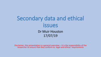
Illustration: Research Question 1Results with weighting only (no variance adjustment)Results with no weighting and no variance adjustment*Results are for illustration purposes only; please do not cite or distribute.
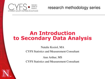
Illustration: Research Question 2 Conduct 2nd order (quadratic) latent growth model in Mplus
Illustration: Research Question 2*Results are for illustration purposes only; please do not cite or distribute.
Illustration: Research Question 2
Other Considerations
Training Opportunities 2-5 day government- or other institution-sponsored workshops– AERA Institute on Statistical Analysis & AERA Faculty Institute http://www.aera.net/grantsprogram/res training/stat institute/SIFly.html http://www.aera.net/grantsprogram/res training/stat institute/SIFacFly.html– IES sponsored workshops http://ies.ed.gov/whatsnew/conferences/?cid 2– AIR http://airweb.org/?page 1803 ICPSR 1 week offerings– http://www.icpsr.umich.edu/icpsrweb/sumprog/ 1 day pre-annual meeting workshops– E.g., “Early Childhood Surveys at NCES: The ECLS and NHES DataUsers Workshop” (2011 SRCD biennial meeting)
Funding Opportunities AERA Dissertation and Research Grants– http://www.aera.net/grantsprogram/ NIH Grants– http://grants.nih.gov/grants/guide/– E.g., “R40 Maternal & Child Health Research Secondary DataAnalysis Studies Grants”– R21 grant mechanism (exploration) IES Grants (exploration; Goal 1)– http://ies.ed.gov/funding/– NAEP Secondary Analysis Grants– RFP‟s that encourage use of secondary data, for example, the“Social and Behavioral Context for Academic Learning” RFP AIR Grants– http://www.airweb.org/?page 1622
ReferencesAIR, NCES, & NSF (2011). National Summer Data Policy Institute training materials.Washington, D.C.Asparouhov, T., & Muthén, B. (2010). Plausible values for latent variables using Mplus.Technical Report. www.statmodel.comBoslaugh, S. (2007). Secondary data sources for public health: A practical guide. NewYork, NY: Cambridge.Enders, C. K. (2010). Applied missing data analysis. New York, NY: Guilford.Lohr, S. L. (2010). Sampling: Design and analysis (2nd Ed.). Boston, MA: Brooks/Cole.Kiecolt, K. J., & Nathan, L. E. (1985). Secondary analysis of survey data. Newbury Park,CA: SAGE.Kish, L. (1965). Survey sampling. New York: Wiley.McCall, R. B., & Appelbaum, M. I. (1991). Some issues of conducting secondary analyses.Developmental Psychology, 27, 911-917.Mislevy, R. J., Beaton, A. E., Kaplan, B., & Sheehan, K. M. (1992). Estimating populationcharacteristics from sparse matrix samples of item responses. Journal of EducationalMeasurement, 29, 133-161.NCES (2011). ECLS-B database training seminar materials. Washington, D.C.
ReferencesSpagat, M., & Dougherty, J. (2010). Conflict deaths in Iraq: A methodological critique ofthe ORB survey estimate. Survey Research Methods, 4, 3-15.Thomas, S. L., & Heck, R. H. (2001). Analysis of large-scale secondary data in highereducation research: Potential perils associated with complex sampling designs.Research in Higher Education, 42, 517-540.Tourangeau, K., Nord, C., Lê, T., Sorongon, A. G., & Najarian, M. (2009). Early ChildhoodLongitudinal Study, Kindergarten Class of 1998-99 (ECLS-K), Combined User’sManual for the ECLS-K Eighth-Grade and K-8 Full Sample Data Files and ElectronicCodebooks (NCES 2009-004). National Center for Education Statistics, Institute ofEducation Sciences, U.S. Department of Education. Washington, DC.Trzesniewski, K. H., Donnellan, M. B., & Lucas, R. E. (Eds) (2011). Secondary dataanalysis: An introduction for psychologists. Washington, D.C.: APA.Vartanian, T. P. (2011). Secondary data analysis. New York, NY: Oxford.
Thanks!For more information, please contact:Natalie Koziol, nak371@neb.rr.com
Taylor series linearization method –Involves specifying cluster and stratum variables Replication methods –Balanced repeated replication (BRR) –Jackknife replication (JK1, JK2, JKn) –Choice of method depends on samplin