Transcription
A Concise Introduction to Astrophysics– Lecture Notes for FY2450 –M. Kachelrieß
M. KachelrießInstitutt for fysikkNTNU, TrondheimNorwayemail: Michael.Kachelriess@ntnu.noc M. Kachelrieß 2008, minor corrections 2011.Copyright
ContentsIStellar astrophysics101 Continuous radiation from stars1.1 Brightness of stars . . . . . . . . . . . . . . . .1.2 Color of stars . . . . . . . . . . . . . . . . . . .1.3 Black-body radiation . . . . . . . . . . . . . . .1.3.1 Kirchhoff-Planck distribution . . . . . .1.3.2 Wien’s displacement law . . . . . . . . .1.3.3 Stefan-Boltzmann law . . . . . . . . . .1.3.4 Spectral energy density of a photon gas1.4 Stellar distances . . . . . . . . . . . . . . . . .1.5 Stellar luminosity and absolute magnitude scale.111112121314151617182 Spectral lines and their formation2.1 Bohr-Sommerfeld model for hydrogen-like atoms . . . . . . . . . . . . . . . .2.2 Formation of spectral lines . . . . . . . . . . . . . . . . . . . . . . . . . . . . .2.3 Hertzsprung-Russel diagram . . . . . . . . . . . . . . . . . . . . . . . . . . . .202022233 Telescopes and other detectors3.1 Optical telescopes . . . . . . . . . . . .3.1.1 Characteristics of telescopes . . .3.1.2 Problems and limitations . . . .3.2 Other wave-length ranges . . . . . . . .3.3 Going beyond electromagnetic radiation3.3.1 Neutrinos . . . . . . . . . . . . .3.3.2 Gravitational waves . . . . . . .26262628283031314 Basic ideas of special relativity4.1 Time dilation – a Gedankenexperiment . .4.2 Lorentz transformations and four-vectors .4.2.1 Galilean transformations . . . . . .4.2.2 Lorentz transformations .4.2.3 Energy and momentum . . . . . .4.2.4 Doppler effect . . . . . . . . . . . .323232323334345 Binary stars and stellar parameters5.1 Kepler’s laws . . . . . . . . . . . . . . . . . . . . . . . . . . . . . . . . . . . .5.1.1 Kepler’s second law: The area law . . . . . . . . . . . . . . . . . . . .5.1.2 Kepler’s first law . . . . . . . . . . . . . . . . . . . . . . . . . . . . . .363638394
Contents.404041426 Stellar atmospheres and radiation transport6.1 The Sun as typical star . . . . . . . . .6.2 Radiation transport . . . . . . . . . . .6.3 Diffusion and random walks . . . . . . .6.4 Photo-, chromosphere and corona . . . .43434345467 Main sequence stars and their structure7.1 Equations of stellar structure . . . . . . . . . . . . . .7.1.1 Mass continuity and hydrostatic equilibrium . .7.1.2 Gas and radiation pressure . . . . . . . . . . .7.1.3 Virial theorem . . . . . . . . . . . . . . . . . .7.1.4 Stability of stars . . . . . . . . . . . .7.1.5 Energy transport . . . . . . . . . . . . . . . . .7.1.6 Thermal equilibrium and energy conservation .7.2 Eddington luminosity and convective instability . . . .7.3 Eddington or standard model . . . . . . . . . . . . . .7.3.1 Heuristic derivation of L M 3 . . . . . . . . .7.3.2 Analytical derivation of L M 3 . . .7.3.3 Lifetime on the Main-Sequence . . . . . . . . .7.4 Stability of stars . . . . . . . . . . . . . . . . . . . . .7.5 Variable stars – period-luminosity relation of Cepheids7.6 Exercises . . . . . . . . . . . . . . . . . . . . . . . . .48484849505152545455555557585858. . . . . . . . . . . . . . . . . . . . . . . .59595959606162636363656568.70707172735.25.35.1.3 Kepler’s third law . . .Determining stellar masses . . .5.2.1 Mass-luminosity relationStellar radii . . . . . . . . . . .8 Nuclear processes in stars8.1 Possible energy sources of stars . . . . . . . . . . . . . . . .8.1.1 Gravitational energy . . . . . . . . . . . . . . . . . .8.1.2 Chemical reactions . . . . . . . . . . . . . . . . . . .8.1.3 Nuclear fusion . . . . . . . . . . . . . . . . . . . . .8.2 Excursion: Fundamental interactions . . . . . . . . . . . . .8.3 Thermonuclear reactions and the Gamov peak . . . . . . .8.4 Main nuclear burning reactions . . . . . . . . . . . . . . . .8.4.1 Hydrogen burning: pp-chains and CNO-cycle . . . .8.4.2 Later phases . . . . . . . . . . . . . . . . . . . . . .8.5 Standard solar model and helioseismology . . . . . . . . . .8.6 Solar neutrinos . . . . . . . . . . . . . . . . . . . . . . . . .8.6.1 Solar neutrino problem and neutrino oscillations9 End9.19.29.39.4points of stellar evolutionObservations of Sirius B . . . . . . . .Pressure of a degenerate fermion gas .White dwarfs and Chandrasekhar limitSupernovae . . . . . . . . . . . . . . .5
Contents9.5Pulsars . . . . . . . . . . . . . . . . . . . . . . . . . . . . . . . . . . . . . . . .10 Black holes10.1 Basic properties of gravitation . . . . . . . . . . . . .10.2 Schwarzschild metric . . . . . . . . . . . . . . . . . .10.2.1 Heuristic derivation . . . . . . . . . . . . . .10.2.2 Interpretation and consequences . . . . . . .10.3 Gravitational radiation from pulsars . . . . . . . . .10.4 Thermodynamics and evaporation of black holesII. . . . . . . . . . . .Galaxies75787878798081838611 Interstellar medium and star formation11.1 Interstellar dust . . . . . . . . . . .11.2 Interstellar gas . . . . . . . . . . .11.3 Star formation . . . . . . . . . . .11.3.1 Jeans length and mass . . .11.3.2 Protostars . . . . . . . . . .878788898991. . . . . . . . . . . . .clusters.929294979813 Galaxies13.1 Milky Way . . . . . . . . . . . . . . . . . . .13.1.1 Rotation curve of the Milkyway . . . .13.1.2 Black hole at the Galactic center . . .13.2 Normal and active galaxies . . . . . . . . . .13.3 Normal Galaxies . . . . . . . . . . . . . . . .13.3.1 Hubble sequence . . . . . . . . . . . .13.3.2 Dark matter in galaxies . . . . . . . .13.3.3 Galactic evolution . . . . . . . . . . .13.4 Active Galaxies and non-thermal radiation . .13.4.1 Non-thermal radiation . . . . . . . . .13.4.2 Radio galaxies . . . . . . . . . . . . .13.4.3 Other AGN types and unified picture.99999910110210310310410610710710911012 Cluster of stars12.1 Overview . . . . . . . . . . . . .12.2 Evolution of a globular cluster .12.3 Virial mass . . . . . . . . . . . .12.4 Hertzsprung-Russell diagrams for.III Cosmology11314 Overview: Universe on large scales14.1 Problems of a static, Newtonian Universe14.2 Einstein’s cosmological principle . . . . .14.3 Expansion of the Universe: Hubble’s law .14.3.1 Cosmic distance ladder . . . . . .1141141141151166.
Contents15 Cosmological models for an homogeneous, isotropic universe15.1 Friedmann-Robertson-Walker metric for an homogeneous, isotropic15.2 Friedmann equation from Newton’s and Hubble’s laws . . . . . . .15.2.1 Friedmann equation . . . . . . . . . . . . . . . . . . . . . .15.2.2 Local energy conservation and acceleration equation . . . .15.3 Scale-dependence of different energy forms . . . . . . . . . . . . . .15.4 Cosmological models with one energy component . . . . . . . . . .15.5 Determining Λ and the curvature R0 from ρm,0 , H0 , q0 . . . . . . .15.6 The ΛCDM model . . . . . . . . . . . . . . . . . . . . . . . . . . .16 Early universe16.1 Thermal history of the Universe 16.2 Big Bang Nucleosynthesis . . . .16.3 Structure formation . . . . . . .16.4 Cosmic microwave background .16.5 Inflation . . . . . . . . . . . . . .Time-line of important dates. . . . . . . . . . . . . . . . . . . . . . . . . . . . . . . . . . . . . . . . . . . . . . . . . . . . . . . . . . . . . . . . .universe. . . . . . . . . . . . . . . . . . . . . . . . . . . . .118118121121123124125126128.130130132134136137A Some formulae139A.1 Mathematical formulae . . . . . . . . . . . . . . . . . . . . . . . . . . . . . . . 139A.2 Some formulae from cosmology . . . . . . . . . . . . . . . . . . . . . . . . . . 139B Units and useful constantsB.1 SI versus cgs units . . . . . . . . . . . . .B.2 Natural units . . . . . . . . . . . . . . . .B.3 Physical constants and measurements . .B.4 Astronomical constants and measurementsB.5 Other useful quantities . . . . . . . . . . .B.6 Abbreviations: . . . . . . . . . . . . . . .B.7 Properties of main-sequence stars . . . . .1401401401411411411421427
Astrophysics—some introductory remarks Astronomy is with mathematics one of the oldest branches of science. It has served asbasis for calendars, navigation, has been an important input for religions and was for along time intertwined with astrology. Some of the most important steps in modern astronomy were:– Galileo performed 1609 the first astronomical studies using a telescope. He discovered among others four Saturn moons and sun spots.– Kepler (1571-1630) developed his three laws of planetary motions, based on observations of Tycho Brahe.– Newton established 1687 his laws of motion and gravitation.– The measurement of the distance to Venus 1761 and 1769 during its transits ofthe Sun with the help of the first global measurement campaign and to the neareststars 1838 by Bessel using trigonometric parallaxes established the first rungs inthe “cosmic distance ladder.”– Fraunhofer discovered around 570 spectral lines in the solar light in 1814 andcatalogued them. This opened together with the spectral analysis of Kirchhoffand Bunsen (1859) the way to study the physical properties of stars.– Einstein’s general theory of relativity (1916) provided the first consistent basis tostudy cosmology.– The “Great Debate” in 1920 was concerned about the question “Does the MilkyWay represents the whole Universe or is it just one island among many others?”Öpik, Shapley and Hubble showed that the latter is true.– Hubble discovered 1926 that galaxies are recessing and that their velocity is increasing with distance: The universe is expanding and, extrapolating this expansionback in time led to the idea of the “Big Bang.”– Nuclear fusion was suggested in 1920 by Eddington as source for stellar energy, themain principles were worked out after the advent of quantum mechanics by Betheand v. Weizsäcker in the 1930s.– The discovery of the cosmic 2.7 Kelvin background radiation 1964 by Penzias andWilson gave credit to the Big Bang theory. Few other examples for the interconnection of astrophysics and physics, where astronomical observations were an important input for fundamental physics, are:– Olaf C. Römer (1644-1710) showed 1676 that the speed of light is finite by observations of Jupiter moons: Light needs around 20 min to cross the Earth orbit.– The 1919 solar eclipse was the first crucial test passed by the theory of GeneralRelativity of Einstein, while a binary system of two pulsars discovered by Hulseand Taylor in 1974 became the first experimental evidence for the existence ofgravitational waves.8
Contents– Observation of neutrinos from the Sun and produced by cosmic rays in the Earth’satmosphere gave in the 1990’s first firm evidence that neutrinos have non-zeromasses.– The need for a new form of “dark matter” to describe correctly the formation anddynamics of galaxies requires a yet unknown extension of the current standardmodel of elementary particle physics. The same holds true for a new form of ”darkenergy” required for the explanation of the accelerated expansion of the universe. Astronomy as a purely observational science is unique among natural sciences; all othersare based on experiments. Since the observation time is much smaller than the typicaltime scale for the evolution of astronomical objects, we see just a snapshot of the universe. Nevertheless it is possible to reconstruct, e.g., the evolution of stars by studyinglarge samples. On the extragalactic scales, we can use that looking far away meanslooking into the past because of the finite speed of light, while on the cosmological scalewe can use relics formed soon after the Big Bang as testimonies for the state of the earlyuniverse. The “cosmological principle” is based on the belief that the mankind and the Earthhave no special role. Thus physical laws derived on Earth are valid everywhere and atall times. Astronomers and especially cosmologists are said to live these days in a “golden age”:There has been a tremendous increase of knowledge in the last 15 years: Telescopes anddetectors on satellites explore new wavelength ranges, while new automatized ways toanalyse data allow astronomers the comparative study of e.g. millions of galaxies.Astrophysics needs input of practically all sub-disciplines of physics and thus a course onastrophysics cannot be self-contained. However, the course should be accessible to studentswith just a general introduction to physics. Few sections of the text that are somewhat moreadvanced and that can be omitted are marked by stars.I will be glad to receive feedback from the readers of these notes. If you find errors or haveanysuggestions, send me an email!9
Part IStellar astrophysics10
1 Continuous radiation from starsPractically all information we know about stars and galaxies comes from observing electromagnetic radiation, more precisely from two small windows where the Earth atmosphere is(nearly) transparent: The first one is around the range of visible light (plus some windowsin the infra-red (IR)), while the second one is the radio window in the wave-length range1 cm λ 30 m, cf. Fig. 1.1.1.1 Brightness of starsHipparcos and Ptolemy ( 150 B.C.) divided stars into six classes of brightness, called (apparent) magnitudes m: Stars with m 6 were the faintest objects visible by eye, stars withm 1 the brightest stars on the sky. Thus the magnitude scale m increases for fainter objects,a counter-intuitive fact that should be kept in mind.The response of the human eye is not linear but close to logarithmic to ensure a largedynamical range. With the use of photographic plates, the magnitude scale could be definedquantitatively. Pogson found 1856 that the magnitude difference m 5 corresponds to aratio of energy fluxes of F2 /F1 100, where the energy flux F is defined as the energy Egoing through the area A per time t, F E/(At). This ratio was then used as definition,together with m 2.12 for the polar star as reference point. Thus the ratio of received energyper time and area from two stars is connected to their magnitudes byF2 100(m1 m2 )/5 10(m1 m2 )/2.5F1or1m1 m2 2.5 logF1.F2(1.1)(1.2)The modern definition of the magnitude scale does not agree completely with the originalGreek one: For instance, the brightest star visible from the Earth, Sirius, has the magnitudem 1.5 instead of the Ptolemic m 1. Note also that in particular astronomers use oftenthe equivalent name (apparent) brightness b for the energy flux received on Earth from a staror a galaxy.Ex.: The largest ground-based telescopes can detect stars or galaxies with magnitude m 26. Howmuch fainter are they than a m 1 star like Antares?F1 10 25/2.5 10 10 .F2(1.3)Thus the number of photons received per time and frequency interval from such a faint object is afactor 10 10 smaller than from Antares. Since the energy flux F scales with distance r approximately1We denote logarithms to the base 10 with log, while we use ln for the natural logarithm.11
1 Continuous radiation from starsFigure 1.1: Left: The electromagnetic spectrum. Right: Transmission of the Earth’s atmosphere.as 1/r2 , one can say equivalently that with the help of such a telescope one would see a factor 105further than with the bare human eye.This magnitude scale corresponds to the energy flux at Earth, i.e. the scale is not correctedfor the different distance of stars. They are therefore called “apparent magnitudes.”1.2 Color of starsA look at Fig. 1.2 shows that the color of stars and galaxies varies considerably. A quantitativeway to measure the color of stars is to use filters which sensitivity is centered at differentwavelengths λi and compare their relative brightness,mλ1 mλ2 2.5 logFλ1.Fλ2(1.4)Then mλ1 mλ2 is called the color or the color index of the object. Often used are filters forvisible (V), ultraviolet (U), and blue (B) light. For instance, one denotes briefly with B-Vthe difference in magnitudes measured with a filter for blue and visible light,B V mB mV 2.5 logFB.FV(1.5)It is intuitively clear that the color of a star is connected to its temperature—this connectionwill be made more precise in the next section. The color magnitudes are normalized suchthat their differences mλ1 mλ2 are zero for a specific type of stars with surface temperatureT 10, 000 K (cf. Sec. 2.2).1.3 Black-body radiationA black body is the idealization of a medium that absorbs all incident radiation. This idealization is very useful, because many objects close to thermal equilibrium, in particular stars,emit approximately blackbody radiation. In practise, black-body radiation can be approximated by radiation escaping a small hole in a cavity whose walls are in thermal equilibrium.Inside such a cavity, a gas of photons in thermal equilibrium exists.12
1.3 Black-body radiationFigure 1.2: An excerpt from the Deep Field View taken by the Hubble Space Telescope.1.3.1 Kirchhoff-Planck distributionPlanck found empirically 1900 the so-called Kirchhoff-Planck (or simply Planck) distributionBν dν 12hν 3dν2hνc exp( kT ) 1(1.6)describing the amount of energy emitted into the frequency interval [ν, ν dν] and the solidangle dΩ per unit time and area by a body in thermal equilibrium. The function Bν dependsonly on the temperature T of the body (apart from the natural constants k, c and h) and isshown in Fig. 1.4 for different temperature T . The dimension of Bν in the cgs system of unitsiserg.(1.7)[Bν ] Hz cm2 s srIn general, the amount of energy per frequency interval [ν, ν dν] and solid angle dΩ crossingthe perpendicular area A per time is called the (differential) intensity Iν , cf. Fig. 1.3,Iν dE.dν dΩ dA dt(1.8)For the special case of the blackbody radiation, the differential intensity is given by theKirchhoff-Planck distribution, Iν Bν .Equation (1.6) gives the spectral distribution of black-body radiation as function of thefrequency ν. In order to obtain the corresponding formula as function of the wavelength λ,one has to re-express both Bν and dν: With λ c/ν and thus dλ c/ν 2 dν, it followsBλ dλ 2hc21dλ .5hcλ exp( λkT ) 1(1.9)13
1 Continuous radiation from starsdΩdΩϑϑdAdAcos ϑdAcos ϑdAFigure 1.3: Left: A detector with surface element dA on Earth measuring radiation comingfrom a direction with zenith angle ϑ. Right: An imaginary detector on the surfaceof a star measuring radiation emitted in the direction ϑ.The Kirchhoff-Planck distribution contains as its two limiting cases Wien’s law for highfrequencies, hν kT , and the Rayleigh-Jeans law for low-frequencies hν kT . In theformer limit, x hν/(kT ) 1, and we can neglect the 1 in the denominator of the Planckfunction,2hν 3Bν 2 exp( hν/kT ) .(1.10)cThus the number of photons with energy hν much larger than kT is exponentially suppressed.In the opposite limit, x hν/(kT ) 1, and ex 1 (1 x . . .) 1 x. Hence Planck’sconstant h disappears from the expression for Bν , if the energy hν of a single photon is smallcompared to the thermal energy kT and one obtains,Bν 2ν 2 kT.c2(1.11)The Rayleigh-Jeans law shows up as straight lines left from the maxima of Bν in Fig. 1.4.1.3.2 Wien’s displacement lawWe note from Fig. 1.4 two important properties of Bν : Firstly, Bν as function of the frequencyν has a single maximum. Secondly, Bν as function of the temperature T is a monotonicallyincreasing function for all frequencies: If T1 T2 , then Bν (T1 ) Bν (T2 ) for all ν. Bothproperties follow directly from taking the derivative with respect to ν and T . In the formerc2case, we look for the maximum of f (ν) 2hBν as function of ν. Hence we have to find thezeros of f ′ (ν),hν3(ex 1) x expx 0withx .(1.12)kTThe equation ex (3 x) 3 has to be solved numerically and has the solution x 2.821.Thus the intensity of thermal radiation is maximal for xmax 2.821 hνmax /(kT ) orcT 0.50K cmνmax14orνmax 5.9 1010 Hz/K .T(1.13)
1.3 Black-body radiationBν in [eV cm-2 s-1 sr-1] ?10-15T 104K10-20T 103K10-25T 100K10-301e 081e 091e 101e 11ν in Hz1e 121e 13Figure 1.4: The Planck distribution Bν as function of the frequency ν for three differenttemperatures.Similarly one derives, using the expression for Bλ , the value λmax where Bλ peaks asλmax T 0.29K cm .(1.14)This equation is called Wien’s displacement law. Thus determining the color of a star tellsus its temperature: A hot star is bluish and a cool star reddish. In practise, the maximum ofthe Planck distribution lies often outside the range of visible light and the measurement of acolor index like U V is an easier method to determine the temperature T of a star.Ex.: Surface temperature of the Sun:We can obtain a first estimate of the surface temperature of the Sun from the know sensitivity ofthe human eye to light in the range 400–700 nm. Assuming that the evolution worked well, i.e. thatthe human eye uses optimal the light from the Sun, and that the atmosphere is for all frequenciesin the visible range similarly transparent, we identify the maximum in Wien’s law with the centerof the frequency range visible for the human eye. Thus we set λmax, 550 nm, and obtain T 2.9 106 nm K/550 nm 5270 K for the surface temperature of the Sun.This simple estimate should be compared to the precise value of 5781 K for the “effective temperature”of the solar photosphere defined in the next subsection.1.3.3 Stefan-Boltzmann lawIntegrating Eq. (1.6) over all frequencies and possible solid angles gives the energy flux Femitted per surface area A by a black body. The angular integral consists of the solid angledΩ dϑ sin ϑdφ and the factor cos ϑ taking into account that only the perpendicular areaA A cos ϑ is visible,ZdΩ cos ϑ Z02πdφZπ/2dϑ sin ϑ cos ϑ π0Zπ/2dϑ sin 2ϑ π .(1.15)015
1 Continuous radiation from starsϑdAdlFigure 1.5: The connection between the contained energy density u and the intensity I ofradiation crossing the volume dV .Next we perform the integral over dν substituting x hν/(kT ),F πwhere we usedR 0x3 dxex 1Z dνBν 02π(kT )4c2 h3Z0 x3 dx σT 4 ,ex 1(1.16) π 4 /15 and introduced the Stefan-Boltzmann constant,σ erg2π 5 k 4 5.670 10 5 2 4 .2315c hcm K s(1.17)If the Stefan-Boltzmann law is used to define the temperature of a body that is only approximately in thermal equilibrium, T is called effective temperature Te .1.3.4 Spectral energy density of a photon gasA light ray crosses an infinitesimal cylinder with volume dV dAdl in the time dt dl/(c cos ϑ), cf. Fig. 1.5. Hence the spectral energy density uν of photons, i.e. the number ofphotons per volume and energy interval, in thermal black-body radiation isZdE4πdE1uν dΩ Bν Bν .(1.18)dV dνc cos ϑdtdAdνccThe (total) energy density of photons u follows asZ4π dνBν aT 4 ,u c 0(1.19)where we introduced the radiation constant a. Comparing with Eqs. (1.16) and (1.17) showsthat a 4σ/c.Ex.: Calculate the density and the mean energy of the photons in thermal black-body radiation attemperature T .16
1.4 Stellar distances starUUUUp UUUUUUUUUUUUUUU UUxUU EarthSun ϑdxFigure 1.6: Measurement of the trigonometric parallax. Left: The apparent movement of anearby star during a year: Half of this angular difference is called the parallaxangle or simply the parallax p. Right: Indirect determination of the Earth-Sundistance.The number density of black-body photons is connected to the energy density by the replacementBν Bν /(hν),4πn cZ0 Bν8πdν 3hνcZ0 ν28πdν 3 (kT /h)3hνc) 1exp( kTZ0 x22ζ(3)dx x e 1π2µkT c¶3,where we looked up the result for the last integral in Table A.1. The mean energy of photons attemperature T follows then ashEi hhνi π4u kT 2.701kT .n30ζ(3)1.4 Stellar distancesRelatively nearby stars are seen at slightly different positions on the celestial sphere (i.e. thebackground of stars that are “infinitely” far away) as the Earth moves around the Sun. Halfof this angular difference is called the parallax angle or simply the parallax p. From Fig. 1.6,one can relate the mean distance AU of the Earth to the Sun, the parallax p and the distanced to the star byAUtan p .(1.20)d17
1 Continuous radiation from starsWith tan p p for p 1, one has d 1/p. Because of this simple and for observationsimportant relation, a new length unit is introduced: The parsec is defined to be the distancefrom the Earth to a star that has a parallax of one arcsecond2 . Thusd[pc] 1p[′′ ](1.21)i.e. a star with a parallax angle of n arcseconds has a distance of 1/n parsecs. Since onearcsecond is 1/(360 60 60) 1/206265 fraction of 2π, a parsec corresponds to 206 265AU.To express finally the unit pc in a known unit like cm, we have to determine first the EarthSun distance, the astronomical unit AU. As first step one measures the distance d to an innerplanet at the time of its greatest elongation (i.e. the largest angular distance ϑ between theSun and the planet). Nowadays, one uses a radar signal to Venus. Then AU d/ cos ϑ, cf.the right panel of Fig. 1.6, and one finds 1AU 1.496 1013 cm. As result, one determinesone parsec as 1 pc 206, 265 AU 3.086 1018 cm 3.26 lyr.1.5 Stellar luminosity and absolute magnitude scaleThe total luminosity L of a star is given by the product of its surface A 4πR2 and theradiation emitted per area σT 4 ,L 4πR2 σT 4 .(1.22)Since the brightness or energy flux F was defined as F E/(At) L/A, we recover theinverse-square law for the energy flux at the distance r R outside of the star,F L.4πr2(1.23)The validity of the inverse-square law F(r) 1/r2 relies on the assumptions that no radiationis absorbed and that relativistic effects can be neglected. The later condition requires inparticular that the relative velocity of observer and source is small compared to the velocityof light.Ex.: Luminosity and effective temperature of the Sun.The energy flux received from the Sun at the distance of the Earth, d 1 AU, is equal to F 1365 W/m2 . (This energy flux is also called “Solar Constant.”) The solar luminosity L follows thenasL 4πd2 F 4 1033 erg/sand serves as a convenient unit in stellar astrophysics. The Stefan-Boltzmann law can then be usedto define with R 7 1010 cm the effective temperature of the Sun, Te (Sun) T 5780 K.The brightness discussed in Sec. 1.1 is based on the observed energy fluxes on Earth and doesnot account for the different distance of stars. It is therefore called “apparent magnitude”.To compare the intrinsic luminosities of stars, one defines the absolute magnitude M as theone a star would have at the standard distance d 10 pc.2A degree, i.e. the 1/360 part of a circle is divided into 60 arcminutes and 60 60 arcseconds, 360 ′′360 60′ 360 60 60 .18
1.5 Stellar luminosity and absolute magnitude scaleUsing that F 1/d2 , the relation between m and M is from Eq. (1.2)m M 2.5 logµd10pc¶2 5 logd.10pc(1.24)The quantity m M is also called distance modulus.Measuring the received energy flux F from a star with known absolute magnitude establishes also the conversion between M and usual cgs or SI units,L 3.02 1035erg 10 0.4M 3.02 1028 W 10 0.4M .s(1.25)Exercises1. Show that the mean distance between black-body photons corresponds approximately tothe wave-length of photons from the maximum of the Planck distribution, nγ 1/λ3max .2. Derive Wien’s law both for frequency and wavelength. Hint: The equations ex (5 x) 5and ey (3 y) 3 have the solutions x 4.965 and y 2.821. Show that λmax 6 c/νmax .3. Show that Bν (T1 ) Bν (T2 ) for all ν, if T1 T2 .4. Derive the Earth-Sun distance D assuming that both are perfect blackbodies. UseR 7 1010 cm, T 5780 K and T 288 K.19
2 Spectral lines and their formationClassical astronomy was mainly concerned with the determination of planetary orbits – anunderstanding of the physical properties of the Sun or stars in general seemed to be impossible.The breakthrough that paved the way to stellar astrophysics was the spectral analysis ofstellar light: Already Fraunhofer identified one prominent of the dark lines in the continuousspectrum of the Sun with the one emitted by salt sprinkled in a flame.The field of spectral analysis was then established by Kirchhoff and Bunsen in 1859: Theyrealized that each element produces its own pattern of spectral lines and can be therebyidentif
Astronomy as a purely observational science is unique among natural sciences; all others are based on experiments. Since the observation time is much smaller than the typical time scale for the evolution of astronomical objects, we see just a snapshot of the uni-verse. Nevertheless it is