Transcription
Computational Visual Mediahttps://doi.org/10.1007/s41095-021-0209-9Vol. 7, No. 2, June 2021, 169–185Review ArticleA survey on deep learning-based Monte Carlo denoisingYuchi Huo1 , Sung-eui Yoon1 ()c The Author(s) 2021. Abstract Monte Carlo (MC) integration is usedubiquitously in realistic image synthesis because of itsflexibility and generality. However, the integrationhas to balance estimator bias and variance, whichcauses visually distracting noise with low sample counts.Existing solutions fall into two categories, in-processsampling schemes and post-processing reconstructionschemes. This report summarizes recent trends inthe post-processing reconstruction scheme. Recentyears have seen increasing attention and significantprogress in denoising MC rendering with deep learning,by training neural networks to reconstruct denoisedrendering results from sparse MC samples. Manyof these techniques show promising results in realworld applications, and this report aims to provide anassessment of these approaches for practitioners andresearchers.Keywords rendering; Monte Carlo (MC) denoising;deep learning; ray tracing1IntroductionThe synthesis of realistic images of virtual worlds isone of the primary driving forces for the developmentof computer graphics techniques [1, 2]. One ofthe firmly established bases for such a purposeis MC integration [3], which is renowned for itsgenerality and heavy computational consumption.MC integration methods are attractive because oftwo distinct advantages. Firstly, they offer a unifiedframework for rendering almost every physicallybased rendering effect. This significantly reducesthe burden of exhaustive case-by-case customizationof rendering pipelines. Secondly, most MC methodsguarantee mathematical convergence to the ground1 KAIST, Daejeon, 31414, Republic of Korea. E-mail: Y. Huo,huo.yuchi.sc@gmail.com; S.-e. Yoon, sungeui@kaist.edu ( ).Manuscript received: 2020-12-25; accepted: 2021-01-23169truth, which is a critical virtue for high-qualityrendering that requires temporal consistency andphysical fidelity.Classical MC integration methods, however, requirea large number of samples to achieve faithfulconvergence. Despite continuously increasing computational power, the cost of realistic renderingremains a limiting, practical constraint, as it takeshours to render one high-quality image, or frame.When using few samples, MC integration resultsoften suffer from estimator variance, which appears asvisually distracting noise. The heavy computationalconsumption is one of the primary factors prohibitinga wider accessibility of MC integration. To addressthis problem, common approaches either devisemore sophisticated sampling strategies to increasesampling efficiency, or develop local reconstructionfunctions to trade mathematical convergence forvisually appealing denoising. Such a post-processingscheme is known as MC denoising, one of the mostinvestigated areas in the rendering community.Recently, deep learning techniques have earnedunprecedented attention and exceeded manytraditional algorithms in various domains [4, 5].Derived from traditional MC reconstruction [6],MC denoising in combination with deep learningtechniques has achieved notable progress andhas become a topic of interest in recent years.Furthermore, industry has actively embraced thelatest achievements. For example, in the movieindustry, Pixar’s RenderMan [7] adapted adaptivesampling and denoising filters in the production ofToy Story 4. Another example [8] in the gamingindustry generates high-quality images with lowsample counts for real-time use.This report summarizes state-of-the-art techniquesin deep learning-based MC denoising. We start witha direct introduction to the basic concepts and then
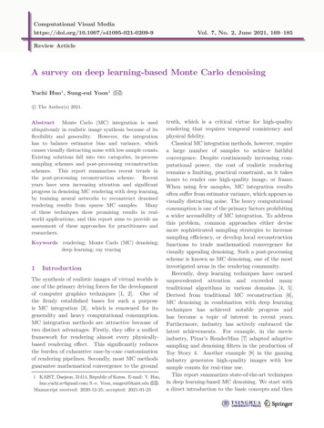
170Y. Huo, S.-e. Yoondiscuss the components of the area in detail (seeSection 2). Afterwards, we provide a comprehensiveoverview which categorizes the related research intothree topics: pixel denoising (Section 3), nontrivial-domain denoising (Section 4), and high-dimensional denoising (Section 5).We conclude this report by summarizing andcomparing the discussed techniques (see Section 6).2Deep learning-based Monte Carlodenoising conceptsClassical MC rendering estimates some target c, e.g.,a pixel’s color, through MC integration, as the sumof the contributions from M samples in some domainΩ, e.g., a pixel: c Ωf (s) ds M1 f (sm )M m 1 p(sm )(1)where f (sm ) and p(sm ) denote the contribution andthe sampling probability of the m-th sample, sm ,on the pixel, respectively. This kind of general MCintegration produces estimation variance with lowsample counts, leading to visually annoying noise.The problem inherently motivates the development ofMC denoising techniques to filter the noisy inputto achieve a plausible rendering quality with areasonable time budget.MC denoising can be formally described as amapping g of an input x to the ground-truth rrendered by a high sample count (Fig. 1). In themost common case, x is a tuple correlated with ashading point p, such as a pixel, as xp {cp , fp },where cp represents noisy values achieved with lowsample counts and fp represents auxiliary features,e.g., surface normal or textures over multiple samplescontributing to p. While using deep learning, thepursuit of optimal g can be formulated as the trainingof a neural network parameterized by a set of weightsθ representing g. Through a supervised learningprocess that utilizes a dataset with N example pairsof (x1 , r1 ), . . . , (xN , rN ), the estimated parameters θ̂are optimized via a loss function asN1 (rn , g(X n ; θ))(2)N n 1where X n is a block of per-pixel vectors in theneighborhood of xn to produce the reconstructedoutput at pixel xn [9]. In reference, the trainednetwork takes seconds or minutes to generate r̂n g(X n ; θ̂), a visually plausible approximation tothe ground-truth that requires hours of rendering.Despite a lack of rigorous analysis of guaranteesof mathematical convergence, this approximationreforms production pipelines by enabling renderingwith a quality visually indistinguishable to the groundtruth, at a much faster speed, and will approachingan interactive rate in the near future.θ̂ min33.1Pixel denoisingApproachesThis section covers the approaches for a basicapplication scenario of MC denoising, thereconstruction of a single smooth image withthe help of auxiliary features and noisy inputs. Theneural networks take as input an image with noisyper-pixel colors, usually samples’ average radianceestimated by path tracing [1], and predict thecorresponding smoothed image. Because the resultsof most MC integration methods can be stacked inimage space, directly denoising the per-pixel colorscan work as a general post-processing add-on toFig. 1 Deep learning-based Monte Carlo denoising method trains a neural network to reduce Monte Carlo noise in input images. Reproducedc Author 2018.with permission from Ref. [9],
A survey on deep learning-based Monte Carlo denoisingexisting rendering pipelines without the need toreorganize data flows. Thus, pixel denoising rapidlybecame a popular solution both in academia andindustry.We categorize the research in pixel denoisingaccording to prediction targets of neural networks,which imply the underlying problem formulation usedby the denoising process. Overall, we categorizethem as performing parameter prediction, radianceprediction, or kernel prediction. Table 1 summarizesthe related papers.3.2Parameter predictionAn early attempt to utilize deep learning in MCdenoising was motivated by a desire to predict optimalparameters of conventional MC filters [10]. Beforethis paper, the most successful MC denoising methodswere based on handcrafted filters using additionalscene features such as shading normals and texturealbedo. The existing challenge was to optimize theparameters, i.e., filter bandwidths, of the filter modelsto reduce noise yet preserve scene details.Kalantari et al. [10] observed that there is a complexrelationship between noisy scene data and ideal filterparameters, and proposed to learn this relationshipthrough deep learning. Their method uses crossbilateral and cross non-local mean filters of variousauxiliary features (world positions, shading normals,texture values, etc.) for the final reconstruction and amultilayer perceptron (MLP) neural network [11–13]to predict optimal weights for each feature in the filter.To use the framework, an MLP is first trained in anoffline process on a set of noisy images of scenes witha variety of distributed effects to regress the optimal171filter parameters that minimize the difference betweenthe reconstructed output and the ground truth. Atrun-time, the trained network can then predict thefilter parameters for new scenes to produce filteredimages in just a few seconds. As shown in Fig. 2,the results were superior to previous approaches ona wide range of distributed effects such as depth offield, motion blur, area lighting, glossy reflections,and global illumination.Xing and Chen [14] also adapted a parameterestimation network to address noise artifacts frompath tracing. The method contains sampling andreconstruction stages. Stein’s unbiased risk estimator(SURE) [15] is adopted to estimate the noise levelper pixel that guides an adaptive sampling process.A modified MLP network is then used to predict theoptimal reconstruction parameters. In the samplingstage, coarse samples are firstly generated, and thena noise level map is estimated with SURE to guideadditional sampling. In the reconstruction stage, themodified MLP network is adopted to predict optimalreconstruction parameters of anisotropic filters forthe final images, using the extracted features.3.3Kernel predictionBased on the observation that predicting parametersof conventional handcrafted filters establishes localreconstruction kernels for pixels in an indirect way,another group of fruitful investigations aimed todirectly predict local reconstruction kernels throughkernel-predicting networks [9, 16, 17].Explicit filters are useful for exploiting conventionalMC denoising models, but may limit denoisingcapability even when using deep neural networks toFig. 2 Result of using the trained network of Kalantari et al. [10] (PPSD) to drive a filter for denoising a new MC rendered image, with across-bilateral filter for the Kitchen scene (1200 800, left) and with a non-local means filter for the San Miguel Hallway scene (800 200, right).Both of these scenes were path-traced and contain severe noise at 4 samples per pixel. The trained network is able to estimate the appropriatec ACM 2015.filter parameters and effectively reduce the noise in only a few seconds. Reproduced with permission from Ref. [10],
172predict the optimal parameters [16]. To address thisproblem, Bako et al. [16] proposed a novel, supervisedlearning approach that allows the filtering kernel tobe more complex and general by leveraging a deepconvolutional neural network (CNN) architecture[18, 19]. The approach introduced a novel, kernelprediction network which employs the CNN toestimate the local weighting kernels used to computeeach denoised pixel from its neighbors. The resultsdemonstrate an improved accuracy compared toparameter-predicting MC denoisers and roughly 5–6 times faster convergence of the weighted kernelprediction than for direct radiance prediction. Othertraining techniques have been widely adopted, andsome of them include decomposition of diffuse andspecular components, separation of albedo fromnetwork prediction, and logarithmic transformationof specular color (Fig. 3).Vogels et al. [9] expanded the capabilities of kernelpredicting networks using asymmetric loss functionsthat are designed to preserve details and provide theuser with direct control over the variance-bias tradeoff during inferencing. They also reconstituted thepipeline with some task-specific modules, includingfour distinct components. First, a source-awareencoder extracts low-level features and embedsthem into a common feature space, enabling quickadaptation of a trained network to novel data. Second,spatial and temporal modules extract abstract, highlevel features for kernel-based reconstruction. Third,a complete network is designed to preserve detailsand provide the user with direct control over thevariance-bias trade-off during inferencing. Fourth, anerror-prediction module infers reconstruction errorY. Huo, S.-e. Yoonmaps for adaptive sampling. This modular designenables a production level MC denoising frameworkin terms of detail preservation, low-frequency noiseremoval, and temporal stability for processing variousproduction and academic datasets. Finally, they shedlight on the academic research by offering a theoreticalanalysis of convergence rates of kernel predictionarchitectures.MC denoisers, also known as biased MC estimators,reduce MC noise by exploring the correlation betweennearby pixels. As a result, they suffer from methodspecific residual noise or systematic errors. Back etal. [20] aimed to mitigate such remaining errors byunifying an independent unbiased estimator and acorrelated biased estimator with a kernel-predictingneural network. Their framework takes a pair ofimages, one with independent estimates, and theother with the corresponding correlated estimatesgenerated by existing MC denoisers. A neuralnetwork is trained to exploit the correlation betweenthese two pixel estimates and output a combinationkernel for the weighted reconstruction of final images.The results of the unified framework outperform bothsingle estimators both visually and numerically.3.4Radiance predictionParameter-predicting and kernel-predicting frameworks generally have achieved great success, but thekernel filtering scheme sometimes imposes restrictionson flexible fusion with state-of-the-art deep learningtechniques. Therefore, another natural evolution of deeplearning-based MC denoising trains neural networksto directly predict per-pixel color, i.e., the outgoingradiance towards the viewpoint at each footprint.Fig. 3 Overview of the kernel-predicting framework [16]. It starts by independently preprocessing diffuse and specular data from the renderingsystem, and then feeds the information to two separate networks to denoise the diffuse and specular illumination, respectively. The output fromeach network undergoes reconstruction (direct reconstruction or weighted reconstruction through the predicted kernels) and postprocessingc Author 2017.before being combined to obtain the final, denoised image. Reproduced with permission from Ref. [16],
A survey on deep learning-based Monte Carlo denoisingWhile most MC denoising methods rely onhandcrafted optimization objectives like MSE orMAPE loss, which do not necessarily ensureperceptually plausible results, Xu et al. [21] presentedan adversarial approach for MC denoising, followingan insight that generative adversarial networks(GANs) [22, 23] can guide neural networks to producemore realistic high-frequency details. The adversarialapproach to evaluate the reconstruction is basedon the Wasserstein distance to measure perceptualsimilarity, which can be interpreted as the distancebetween the denoised and ground truth distributions.In addition, they adapt a feature modulation methodto encode auxiliary features that allow featuresto better take effect at the pixel level, leadingto fine-grained denoising results. Another GANbased denoising method also considers denoisingrendered images from a dataset containing 40 Pixarmovie image frames with added Gaussian noise [24].Because the network does not take auxiliary featuresas input, it can also denoise noisy photographs undernatural light and CT scans.A deep residual network (ResNet) [25] demonstratessignificant improvement over a basic CNN. In orderto take advantage of ResNet, a filter-free directdenoising method based on a standard-and-simpledeep ResNet is trained to remove the noise of MCrendering [26]. The method directly maps the noisyinput pixels to the smoothed output with onlythree common auxiliary features (depth, normal,and albedo), simplifying its integration into mostproduction rendering pipelines. With the helpof ResNet, the simple structure yields comparableaccuracy to other state-of-the-art methods.One distinguishing difference between MCdenoising and natural image denoising is thatauxiliary features, e.g., normals, can be extractedfrom the rendering pipeline, providing noise-freeguidance for image reconstruction. However, theauxiliary features also contain redundant information,which reduces the efficiency of deep learning-basedMC denoising. Yang et al. [27, 28] focused on howto extract useful information from auxiliary features.To address this problem, they first introduced anend-to-end CNN model to fuse feature buffers andpredict a residual radiance map between noisyinput and ground truth to reconstruct a final173image. In addition, a high-dynamic range (HDR)image normalization method is proposed to trainthe model on HDR images in a more efficientand stable way [27]. In follow-up research, theyproposed an autoencoder [29, 30] inspired networkstructure, a dual-encoder network with a featurefusion subnetwork, to first fuse auxiliary features.The fused features and a noisy image are then fed asinputs to a second encoder network to reconstruct aclean image by a decoder network [28]. Compared toconventional solutions using uncompressed auxiliaryfeatures, the method is able to generate satisfactoryresults in a significantly faster way.While deep learning-based MC denoisersdramatically enhance rendering quality, theresults are less reliable when there is insufficientinformation to calculate the features, such as varianceand contrast. To address this issue, Kuznetsovet al. [31] proposed a deep learning approach forjoint adaptive sampling and reconstruction of MCrendering results with extremely low sample counts.In addition to a conventional MC denoising network,they train a CNN to estimate sampling maps forguiding adaptive sample distribution over pixels.Finally, the denoising network produces denoisedimages from the adaptively sampled MC renderingresults.44.1Nontrivial-domain denoisingBackgroundConventional MC denoisers work in image space,where the basic geometric auxiliary features canbe easily extracted from most rendering pipelines.This accessibility makes pixel-based MC denoisers aprevailing choice. However, the physical process oflight transport occurs in a high-dimensional spacewhere some important information is inevitablydegraded when reducing everything into per-pixelradiance. To address this, a research stream aimsto recover the lost information by utilizing variousnontrivial domains, e.g., sample space and gradientdomain, for high-quality rendering of illuminationdetails or challenging effects. This section discusses therelated approaches using nontrivial-domain featuresand their advantages in single-image denoising. Thesummary of these papers is in Table 1.
1744.2Y. Huo, S.-e. YoonSample spaceIn contrast to the traditional pixel-based MC denoisers,Gharbi et al. [17] proposed a sample-based kernelsplatting network. They observed that traditionalMC denoisers exploit summary statistics of a pixel’ssample distributions, which discards much of thesamples’ information and limits their denoising power.The proposed kernel-spatting network, learning themapping between samples and images, embracesunfamiliar network architecture design to solve multiplechallenges associated with the sample space: the orderof the samples is arbitrary, and those samples must betreated in a permutation invariant manner. Insteadof conventional gathering kernels, they suggestedpredicting spatting kernels that splat individual samplesonto nearby pixels using a convolutional neural network.They claimed that, in addition, splatting is a naturalsolution to situations such as motion blur, depth-offield, and many light transport problems, where it iseasier to predict which pixels a sample contributes to,rather than to predict gathering kernels that need todetermine informative relationships between relevantpixels. The new architecture yields higher-qualityresults both visually and numerically for low-samplecount images and distributed-effect images.Per-sample denoisers come with high computationalcosts because of the need to produce kernel weightsand apply a large kernel for each sample in each pixel,which can limit its usability for higher sample counts.Based on this observation, Munkberg and Hasselgren[32] proposed to extract a compact representation ofper-sample information by separating samples intoa fixed number of partitions, called layers in theirpaper, via a data-driven method that learns uniquekernel weights for each pixel in each layer and how tocomposite the filtered layers. This modification givesa practical denoiser the capability to strike a goodtrade-off between cost and quality. Furthermore, itprovides an efficient way to control performance andmemory characteristics, since the algorithm scaleswith the number of layers rather than the numberof samples. Using two partitioned sample layers, thedenoiser achieves interactive rates while producingimage quality similar to larger networks.Assuming that next event estimation (NEE) [33]is used in the rendering process, Lin et al. [34]decomposed the features of Gharbi et al. [17] intosample- and path-space features, where one-bouncepaths are sample-space features and multi-bouncepaths are path-space features. The key insight ofthe separation is to decompose the high-frequencyillumination from short paths and low-frequencyillumination from long paths. The three-scalefeatures—pixel, sample, and path—are combinedto preserve sharp details, using a feature attentionmechanism and feature extractors.4.3Light field spaceMost MC denoisers only use as features the outgoingradiance of samples in each pixel, while each sample isin fact a high-dimensional light path with informationabout the light field [35]. Lin et al. [36] observedthat these methods show powerful denoising ability,but tend to lose geometric or lighting details and toblur sharp features during denoising. Based on thedefinition of the local light field (Fig. 5), the authorsadapted a framework [37] for frequency analysis oflight transport by calculating the frequency contentof the local light field around a given ray. Thelocal light field is defined as a 4D function, withtwo spatial dimensions and two angular dimensions.In the analysis, light transport operations, such astransport in free space or reflection, are transformedFig. 4 Comparison between state-of-the-art pixel-based (Bako et al. [16]) and sample-space (Gharbi et al. [17]) MC denoising algorithms.The sample-space method works with the samples directly, using a splatting approach that makes it possible to appropriately handle variouscomponents of the illumination (indirect lighting, specular reflection, motion blur, depth of field, etc.) more effectively. Reproduced withc ACM 2019.permission from Ref. [17],
A survey on deep learning-based Monte Carlo denoisingFig. 5 The local light field is defined as a 4D function around thecenter ray (ω), parameterized by two spatial coordinates (δx and δy )and two angular coordinates (δθ and δφ ). Reproduced with permissionc IEEE 2020.from Ref. [39], into operations on the Fourier spectrum, thenapproximately represented by the Fourier spectrumof the local light field, the covariance matrix [38]. Aneural network makes use of this covariance matrix, a4 4 matrix encoding the Fourier spectrum of the locallight field at each pixel, to leverage the directionallight transportation information. In addition, theauthor proposed a network extracting feature buffersseparately from the color buffer and then integratedthe two buffers into a shallow kernel predictor.Finally, they suggested an improved loss functionconsidering perceptual loss. These modifications helpto preserve illumination details.Instead of using light-field-space features for imagespace denoising, another category of research aims todirectly reconstruct the denoised incident radiancefield, i.e., the local light field at each pixel, foradvanced goals such as unbiased path guiding [40–42].We cover such works in Section 5.4.4.4Gradient domainGradient-domain rendering methods [43–45] developa common denoising idea of estimating finitedifference gradients of image colors to solve ascreen-space Poisson problem. The gradient-domaininformation is believed to offer additional benefitsbecause of the frequency content of the light transportintegrand and the interplay with the gradientoperator. Recent work combines this long-existingresearch direction with modern CNNs [46]. The newmethod replaces the conventional screened Poissonsolver with a novel dense variant of the U-Netautoencoder, taking auxiliary feature buffers as inputsand using a perceptual image distance metric as lossfunction. The combination significantly improves the175quality obtained from gradient-domain path tracingand yields notably improved image quality comparedto simple image-space MC denoisers.In other independent work, Guo et al. [47] proposedusing a multi-branch autoencoder to replace the Poissonsolver. The network end-to-end learns a mappingfrom a noisy input image and its correspondingimage gradients to a high-quality image with lowvariance. One distinguishing feature of this work isthat the authors train the network in a completelyunsupervised manner by adjusting a non-trivial lossfunction between the noisy inputs and the outputs ofthe network. The loss function combines an energyfunction including a data fidelity term, a gradientfidelity term, and a regularizer constructed fromselected rendering-specific features. In this way, theapproach avoids the tedious and sometimes expensiverendering process to generate noise-free images fortraining, making it a technically unsupervised solution.4.5Photon denoisingWhile path tracing is a general MC integrationapproach for realistic rendering, it is not effectivefor simulating challenging light transport effectslike caustics. Instead, photon mapping [48, 49]has been considered as the method of choice forrendering caustics, but it has not completely adoptedprogress in deep learning techniques. Some recentresearch bridges this gap by training a deep neuralnetwork to predict a kernel function aggregatingphoton contributions at each shading point [50].Photon mapping traces a large number of photonsfrom the light source, and then gathers the photoncontributions at each shading point to achievehigh-quality reconstructions of challenging lighttransportation results which are hard to trace from thecamera. The authors mitigate the required number ofphotons with a network encoding individual photonsinto per-photon features, aggregating them in theneighborhood of a shading point to construct a photonlocal context vector, and inferring a kernel functionfrom the per-photon and photon local context features.This work combines conventional deep learning-baseddenoisers for remaining light transport paths. Theresults show promising high-quality reconstructionsof caustic effects with an order of magnitude fewerphotons than previous photon mapping methodsand significantly outperform path tracing-based MCrendering for caustic effects (Fig. 6).
176Y. Huo, S.-e. YoonFig. 6 Results of photon mapping denoising show high-quality reconstruction of caustic effects [50]. (a,b) Final results of the proposed method(PPSD). (c) Path-tracing results with an image-space denoiser [8]. (d) Results without denoiser. (e) Ground truth. Reproduced with permissionc The Eurographics Association and John Wiley & Sons Ltd. 2020.from Ref. [50], Stochastic progressive photon mapping [51] isan important global illumination method derivedfrom photon mapping. It can simulate causticeffects in a progressive way, but suffers from bothbias and variance with limited iterations, leadingto visually annoying MC noise. Zeng et al. [52]recently proposed a deep learning-based methodspecially designed for denoising the biased renderingsof stochastic progressive photon mapping. Themethod decomposes the light transport into twocomponents, caustic and other, and denoises each partindependently. It also employs additional photonrelated auxiliary features and multi-residual blocksto enhance kernel predicting neural networks.55.1High-dimensional denoisingOverviewSingle-image MC denoisers take as input one noisyimage to produce one high-quality output withoutMC noise. However, such single-image outputdoes not satisfy many applications that requirehigher-dimensional outputs. For example, producingcomputer animation requires a sequence of temporallyconsistent images, and path guiding to generateunbiased rendering results might need to denoisethe whole incident light field at each shading point.In such scenarios, pixel-based MC denoisers are nolonger adequate to generate the high-dimensionaloutputs without special designs for high-dimensionalsignal processing and consistency constraints. Herewe categorize deep learning-based MC denoiserstargeting high-dimensional applications into threetypes, temporal rendering, volume rendering, andradiance field reconstruction, and discuss each indetail. The related papers are summarized in Table 1.5.2Temporal renderingOne of the most important MC rendering applicationsis to generate a sequence of images for computeranimation or interactive applications. Among manysingle-image denoisers, some focus on renderingquality, and others pay additional attention tothe balance between quality and speed to achievean interactive processing rate.Besides speed,an essential consideration is to enhance temporalstability between frames, to avoid low-frequencyvariances that may lead to flicking artifacts inanimation. Pioneering research in this area wasinspired by the good results achieved by recurrentneural networks (RNNs) [53, 54] in the contextof video super-resolution and sub-pixel CNNs, anddescribes an RNN-based framework that dramaticallyimproves temp
per pixel that guides an adaptive sampling process. A modified MLP network is then used to predict the optimal reconstruction parameters. In the sampling stage, coarse samples are firstly generated, and then a noise level map is estimated with SURE to gu