WIXLIB

2.1 Graphical Modeling273in diverse areas of stochastic modeling, including coding theory [89],computer vision [41], knowledge representation [103], Bayesian statistics [40], and natural-language processing [11, 63].Distributions over many variables can be expensive to representnaı̈vely. For example, a table of joint probabilities of n binary variables requires storing O(2n ) floating-point numbers. The insight of thegraphical modeling perspective is that a distribution over very manyvariables can often be represented as a product of local functions thateach depend on a much smaller subset of variables. This factorizationturns out to have a close connection to certain conditional independence relationships among the variables — both types of informationbeing easily summarized by a graph. Indeed, this relationship betweenfactorization, conditional independence, and graph structure comprisesmuch of the power of the graphical modeling framework: the conditional independence viewpoint is most useful for designing models,and the factorization viewpoint is most useful for designing inferencealgorithms.In the rest of this section, we introduce graphical models from boththe factorization and conditional independence viewpoints, focusing onthose models which are based on undirected graphs. A more detailedmodern treatment of graphical modeling and approximate inference isavailable in a textbook by Koller and Friedman [57].2.1.1Undirected ModelsWe consider probability distributions over sets of random variables Y .We index the variables by integers s 1, 2, . . . Y . Every variable Ys Ytakes outcomes from a set Y, which can be either continuous or discrete,although we consider only the discrete case in this survey. An arbitraryassignment to Y is denoted by a vector y. Given a variable Ys Y , thenotation ys denotes the value assigned to Ys by y. The notation 1{y y }denotes an indicator function of y which takes the value 1 when y y and 0 otherwise. We also require notation for marginalization. For a fixed-variable assignment ys , we use the summation y\ys to indicatea summation over all possible assignments y whose value for variableYs is equal to ys .

274ModelingSuppose that we believe that a probability distribution p of interestcan be represented by a product of factors of the form Ψa (ya ) wherea is an integer index that ranges from 1 to A, the number of factors.Each factor Ψa depends only on a subset Ya Y of the variables. Thevalue Ψa (ya ) is a non-negative scalar that can be thought of as a measure of how compatible the values ya are with each other. Assignmentsthat have higher compatibility values will have higher probability. Thisfactorization can allow us to represent p much more efficiently, becausethe sets Ya may be much smaller than the full variable set Y .An undirected graphical model is a family of probability distributions that each factorize according to a given collection of factors.Formally, given a collection of subsets {Ya }Aa 1 of Y , an undirectedgraphical model is the set of all distributions that can be written asp(y) A1 Ψa (ya ),Z(2.1)a 1for any choice of factors F {Ψa } that have Ψa (ya ) 0 for all ya .(The factors are also called local functions or compatibility functions.)We will use the term random field to refer to a particular distributionamong those defined by an undirected model.The constant Z is a normalization factor that ensures the distribution p sums to 1. It is defined asZ A Ψa (ya ).(2.2)y a 1The quantity Z, considered as a function of the set F of factors, isalso called the partition function. Notice that the summation in (2.2) isover the exponentially many possible assignments to y. For this reason,computing Z is intractable in general, but much work exists on how toapproximate it (see Section 4).The reason for the term “graphical model” is that the factorization factorization (2.1) can be represented compactly by means of agraph. A particularly natural formalism for this is provided by factorgraphs [58]. A factor graph is a bipartite graph G (V, F, E) in whichone set of nodes V {1, 2, . . . , Y } indexes the random variables in themodel, and the other set of nodes F {1, 2, . . . , A} indexes the factors.

2.1 Graphical Modeling275The semantics of the graph is that if a variable node Ys for s V isconnected to a factor node Ψa for a F , then Ys is one of the arguments of Ψa . So a factor graph directly describes the way in which adistribution p decomposes into a product of local functions.We formally define the notion of whether a factor graph “describes”a given distribution or not. Let N (a) be the neighbors of the factor withindex a, i.e., a set of variable indices. Then:Definition 2.1. A distribution p(y) factorizes according to a factorgraph G if there exists a set of local functions Ψa such that p can bewritten as Ψa (yN (a) )(2.3)p(y) Z 1a FA factor graph G describes an undirected model in the same waythat a collection of subsets does. In (2.1), take the collection of subsetsto be the set of neighborhoods {YN (a) a F }. The resulting undirected graphical model from the definition in (2.1) is exactly the set ofall distributions that factorize according to G.For example, Figure 2.1 shows an example of a factor graphover three random variables. In that figure, the circles are variablenodes, and the shaded boxes are factor nodes. We have labelled thenodes according to which variables or factors they index. This factor graph describes the set of all distributions p over three variablesthat can be written as p(y1 , y2 , y3 ) Ψ1 (y1 , y2 )Ψ2 (y2 , y3 )Ψ3 (y1 , y3 ) forall y (y1 , y2 , y3 ).There is a close connection between the factorization of a graphicalmodel and the conditional independencies among the variables in itsdomain. This connection can be understood by means of a differentFig. 2.1 An example of a factor graph over three variables.

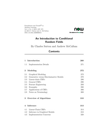
276Modelingundirected graph, called a Markov network, which directly representsconditional independence relationships in a multivariate distribution.Markov networks are graphs over random variables only, rather thanrandom variables and factors. Now let G be an undirected graph overintegers V {1, 2, . . . , Y } that index each random variable of interest.For a variable index s V , let N (s) denote its neighbors in G. Then wesay that a distribution p is Markov with respect to G if it satisfies thelocal Markov property: for any two variables Ys , Yt Y , the variable Ysis independent of Yt conditioned on its neighbors YN (s) . Intuitively,this means that YN (s) on its own contains all of the information that isuseful for predicting Ys .Given a factorization of a distribution p as in (2.1), a correspondingMarkov network can be constructed by connecting all pairs of variablesthat share a local function. It is straightforward to show that p isMarkov with respect to this graph, because the conditional distributionp(ys yN (s) ) that follows from (2.1) is a function only of variables thatappear in the Markov blanket.A Markov network has an undesirable ambiguity from the factorization perspective. Consider the three-node Markov network in Figure 2.2(left). Any distribution that factorizes as p(y1 , y2 , y3 ) f (y1 , y2 , y3 ) forsome positive function f is Markov with respect to this graph. However, we may wish to use a more restricted parameterization, wherep(y1 , y2 , y3 ) f (y1 , y2 )g(y2 , y3 )h(y1 , y3 ). This second model family isa strict subset of the first, so in this smaller family we might notrequire as much data to accurately estimate the distribution. Butthe Markov network formalism cannot distinguish between these twoFig. 2.2 A Markov network with an ambiguous factorization. Both of the factor graphs atright factorize according to the Markov network at left.

2.1 Graphical Modeling277parameterizations. In contrast, the factor graph depicts the factorization of the model unambiguously.2.1.2Directed ModelsWhereas the local functions in an undirected model need not have adirect probabilistic interpretation, a directed graphical model describeshow a distribution factorizes into local conditional probability distributions. Let G be a directed acyclic graph, in which π(s) are the indicesof the parents of Ys in G. A directed graphical model is a family ofdistributions that factorize as:p(y) S p(ys yπ(s) ).(2.4)s 1We refer to the distributions p(ys yπ(s) ) as local conditional distributions. Note that π(s) can be empty for variables that have no parents.In this case p(ys yπ(s) ) should be understood as p(ys ).It can be shown by induction that p is properly normalized. Directedmodels can be thought of as a kind of factor graph in which the individual factors are locally normalized in a special fashion so that (a) thefactors equal conditional distributions over subsets of variables, and(b) the normalization constant Z 1. Directed models are often usedas generative models, as we explain in Section 2.2.3. An example of adirected model is the naive Bayes model (2.7), which is depicted graphically in Figure 2.3 (left). In those figures, the shaded nodes indicatevariables that are observed in some data set. This is a convention thatwe will use throughout this survey.2.1.3Inputs and OutputsThis survey considers the situation in which we know in advance whichvariables we will want to predict. The variables in the model will bepartitioned into a set of input variables X that we assume are alwaysobserved, and another set Y of output variables that we wish to predict.For example, an assignment x might represent a vector of each wordthat occurs in a sentence, and y a vector of part of speech labels foreach word.

278ModelingWe will be interested in building distributions over the combinedset of variables X Y , and we will extend the previous notation inorder to accommodate this. For example, an undirected model over Xand Y would be given byp(x, y) A1 Ψa (xa , ya ),Z(2.5)a 1where now each local function Ψa depends on two subsets of variablesXa X and Ya Y . The normalization constant becomes Ψa (xa , ya ),(2.6)Z x,y a Fwhich now involves summing over all assignments both to x and y.2.2Generative versus Discriminative ModelsIn this section we discuss several examples of simple graphical modelsthat have been used in natural language processing. Although theseexamples are well-known, they serve both to clarify the definitions inthe previous section, and to illustrate some ideas that will arise againin our discussion of CRFs. We devote special attention to the hiddenMarkov model (HMM), because it is closely related to the linear-chainCRF.One of the main purposes of this section is to contrast generativeand discriminative models. Of the models that we will describe, two aregenerative (the naive Bayes and HMM) and one is discriminative (thelogistic regression model). Generative models are models that describehow a label vector y can probabilistically “generate” a feature vector x.Discriminative models work in the reverse direction, describing directlyhow to take a feature vector x and assign it a label y. In principle, eithertype of model can be converted to the other type using Bayes’s rule, butin practice the approaches are distinct, each with potential advantagesas we describe in Section 2.2.3.2.2.1ClassificationFirst we discuss the problem of classification, that is, predicting a singlediscrete class variable y given a vector of features x (x1 , x2 , . . . , xK ).

2.2 Generative versus Discriminative Models279One simple way to accomplish this is to assume that once the classlabel is known, all the features are independent. The resulting classifieris called the naive Bayes classifier. It is based on a joint probabilitymodel of the form:p(y, x) p(y)K p(xk y).(2.7)k 1This model can be described by the directed model shown in Figure 2.3(left). We can also write this model as a factor graph, by defining afactor Ψ(y) p(y), and a factor Ψk (y, xk ) p(xk y) for each feature xk .This factor graph is shown in Figure 2.3 (right).Another well-known classifier that is naturally represented as agraphical model is logistic regression (sometimes known as the maximum entropy classifier in the NLP community). This classifier canbe motivated by the assumption that the log probability, log p(y x), ofeach class is a linear function of x, plus a normalization constant.1 Thisleads to the conditional distribution: K 1(2.8)θy,j xj ,p(y x) exp θy Z(x)j 1 where Z(x) y exp{θy Kj 1 θy,j xj } is a normalizing constant, andθy is a bias weight that acts like log p(y) in naive Bayes. Rather thanusing one weight vector per class, as in (2.8), we can use a differentnotation in which a single set of weights is shared across all the classes.The trick is to define a set of feature functions that are nonzero onlyyxyxFig. 2.3 The naive Bayes classifier, as a directed model (left), and as a factor graph (right).1 Bylog in this survey we will always mean the natural logarithm.

280Modelingfor a single class. To do this, the feature functions can be defined asfy ,j (y, x) 1{y y} xj for the feature weights and fy (y, x) 1{y y} forthe bias weights. Now we can use fk to index each feature function fy ,j ,and θk to index its corresponding weight θy ,j . Using this notationaltrick, the logistic regression model becomes:p(y x) K 1θk fk (y, x) .expZ(x)(2.9)k 1We introduce this notation because it mirrors the notation for CRFsthat we will present later.2.2.2Sequence ModelsClassifiers predict only a single class variable, but the true power ofgraphical models lies in their ability to model many variables that areinterdependent. In this section, we discuss perhaps the simplest formof dependency, in which the output variables in the graphical modelare arranged in a sequence. To motivate this model, we discuss anapplication from natural language processing, the task of named-entityrecognition (NER). NER is the problem of identifying and classifyingproper names in text, including locations, such as China; people, suchas George Bush; and organizations, such as the United Nations. Thenamed-entity recognition task is, given a sentence, to segment whichwords are part of an entity, and to classify each entity by type (person,organization, location, and so on). The challenge of this problem isthat many named entity strings are too rare to appear even in a largetraining set, and therefore the system must identify them based onlyon context.One approach to NER is to classify each word independently as oneof either Person, Location, Organization, or Other (meaningnot an entity). The problem with this approach is that it assumesthat given the input, all of the named-entity labels are independent.In fact, the named-entity labels of neighboring words are dependent;for example, while New York is a location, New York Times is anorganization. One way to relax this independence assumption is toarrange the output variables in a linear chain. This is the approach

2.2 Generative versus Discriminative Models281taken by the hidden Markov model (HMM) [111]. An HMM modelsa sequence of observations X {xt }Tt 1 by assuming that there isan underlying sequence of states Y {yt }Tt 1 . We let S be the finiteset of possible states and O the finite set of possible observations,i.e., xt O and yt S for all t. In the named-entity example, eachobservation xt is the identity of the word at position t, and each stateyt is the named-entity label, that is, one of the entity types Person,Location, Organization, and Other.To model the joint distribution p(y, x) tractably, an HMM makestwo independence assumptions. First, it assumes that each statedepends only on its immediate predecessor, that is, each state yt isindependent of all its ancestors y1 , y2 , . . . , yt 2 given the preceding stateyt 1 . Second, it also assumes that each observation variable xt dependsonly on the current state yt . With these assumptions, we can specify anHMM using three probability distributions: first, the distribution p(y1 )over initial states; second, the transition distribution p(yt yt 1 ); andfinally, the observation distribution p(xt yt ). That is, the joint probability of a state sequence y and an observation sequence x factorizes asp(y, x) T p(yt yt 1 )p(xt yt ).(2.10)t 1To simplify notation in the above equation, we create a “dummy”initial state y0 which is clamped to 0 and begins every state sequence.This allows us to write the initial state distribution p(y1 ) as p(y1 y0 ).HMMs have been used for many sequence labeling tasks in naturallanguage processing such as part-of-speech tagging, named-entityrecognition, and information extraction.2.2.3ComparisonBoth generative models and discriminative models describe distributions over (y, x), but they work in different directions. A generativemodel, such as the naive Bayes classifier and the HMM, is a familyof joint distributions that factorizes as p(y, x) p(y)p(x y), that is, itdescribes how to sample, or “generate,” values for features given thelabel. A discriminative model, such as the logistic regression model, is

282Modelinga family of conditional distributions p(y x), that is, the classificationrule is modeled directly. In principle, a discriminative model could alsobe used to obtain a joint distribution p(y, x) by supplying a marginaldistribution p(x) over the inputs, but this is rarely needed.The main conceptual difference between discriminative and generative models is that a conditional distribution p(y x) does not includea model of p(x), which is not needed for classification anyway. Thedifficulty in modeling p(x) is that it often contains many highly dependent features that are difficult to model. For example, in named-entityrecognition, a naive application of an HMM relies on only one feature,the word’s identity. But many words, especially proper names, willnot have occurred in the training set, so the word-identity feature isuninformative. To label unseen words, we would like to exploit otherfeatures of a word, such as its capitalization, its neighboring words, itsprefixes and suffixes, its membership in predetermined lists of peopleand locations, and so on.The principal advantage of discriminative modeling is that it isbetter suited to including rich, overlapping features. To understandthis, consider the family of naive Bayes distributions (2.7). This is afamily of joint distributions whose conditionals all take the “logisticregression form” (2.9). But there are many other joint models, somewith complex dependencies among x, whose conditional distributionsalso have the form (2.9). By modeling the conditional distributiondirectly, we can remain agnostic about the form of p(x). Discriminative models, such as CRFs, make conditional independence assumptionsamong y, and assumptions about how the y can depend on x, but donot make conditonal independence assumptions among x. This pointalso be understood graphically. Suppose that we have a factor graphrepresentation for the joint distribution p(y, x). If we then construct agraph for the conditional distribution p(y x), any factors that dependonly on x vanish from the graphical structure for the conditional distribution. They are irrelevant to the conditional because they are constantwith respect to y.To include interdependent features in a generative model, we havetwo choices. The first choice is to enhance the model to represent dependencies among the inputs, e.g., by adding directed edges among each xt .But this is often difficult to do while retaining tractability. For example,

2.2 Generative versus Disc

Foundations and TrendsR in Machine Learning Vol. 4, No. 4 (2011) 267–373 c 2012 C. Sutton and A. McCallum DOI: 10.1561/2200000013 An Introduction to Conditional Random Fields Charles Sutton1 and Andrew McCallum2 1 School of Informatics, University o