WIXLIB

instead of doing truly productive work. Don’t fall into this trap. Before we close this dialog,there is one important setting to note and that is the section labeled “Net Names”. For now leaveit as it is. We shall revisit this in the future.Figure 1A-5OK, let’s create a circuit and perform a simulation. You should already have a DC voltage sourceon your work space. From the virtual (blue) components tool bars, select two resistors and anearth ground symbol. We shall make a series loop of the three elements with the negative end ofthe power supply at ground. One resistor will need to be rotated 90 degrees (one horizontal andone vertical). In order to wire the items together, simply click on the free lead of one componentand move to the desired lead of another. While moving, Multisim will draw a ghost line.Clicking on the second component will create a proper wire (by default, colored red). Wires arealways drawn along the horizontal and vertical with 90 degree bends, not directly from point topoint. This is the proper way to draw a schematic in the vast majority of cases.It is possible to click on the middle of a wire in order to tie multiple items together. A small nodecircle will be drawn at the connection point. To delete a wire, click on it to select it. You will seea set of small box “handles” around it. To remove the wire, simply hit the Delete key. Note that12Laboratory Manual for Computer Programming

you can also move the wire with those handles if desired. In fact, it is possible to align wires atodd angles with these handles (again, this is not typical).Note that if you move a component, Multisim will automatically move the wires along with it.You do not have to rewire it. Sometimes, especially if components are too close, the wire may bedraw in an odd, looping form. The easiest solution is to simply separate the components a littlemore.Once the components are in place and wired, double-click each component to set their values asshown in Figure 1A-6. If you’re using power rated virtual resistors, also increase their powerrating to one watt, each. We shall then add two the two voltmeters. Please note that it is perfectlyacceptable to change the component values immediately after dragging them onto the workspace; you don’t have to wait until they are wired together. It is suggested, though, that youdecide upon a particular workflow and stick to it otherwise the chances of forgetting to changecomponents from their default values increases.Figure 1A-6To add the voltmeters (XMM1 and XXM2 in Figure 1A-6), select a virtual DMM from the top ofthe Instruments toolbar along the right edge of the screen. Drag this onto the work space andwire it across R1 as shown in Figure 1A-6. Grab a second virtual DMM and repeat the processfor R2. Now double click on the DMMs. Two small windows will pop up (they might overlapeach other, if so, move one over). Select the V (voltage) button and the straight line (DC) buttonon each of them. The circuit is now ready to perform a simulation.Laboratory Manual for Computer Programming13

To start a simulation, you can select the the rocker switch located in the upper right corner of themenu area. This is the virtual on-off switch. Alternately, you can select Run from the Simulatemenu or use the green Run button on the simulation toolbar. In a moment, you should seevoltages appear on the two virtual DMMs. In order to edit the circuit, the simulation must beturned off. So, if we wish to add or delete components, we must remember to “power down” thecircuit just as we would in a real lab. To be safe, do this now.Multisim has a wide variety of virtual instruments. Some of them are fairly simple such as theDMM just used. Other instruments are virtual recreations of real-world test instruments. Forexample, from the Instruments toolbar select the Tektronix Oscilloscope. You may place thisanywhere on your schematic. Now double click on the small icon for this device (XSC1). Arather ornate window opens which appears to be the front panel of a Tektronix TDS 2024oscilloscope, similar to the models you might see in electronics labs, right down to subtleshadows around the knobs! See Figure 1A-7. This has the advantage of immediacy (assumingyou’ve used this type of oscilloscope before), however, it is not the ultimate way to perform asimulation. We will look at even more powerful and flexible ways of creating simulations in thenext exercise. For now, you may wish to delete this new instrument from the work space andthen save the existing schematic. Remember to always save to either your student account or to aUSB drive. Never save directly to the hard drive in lab.Figure 1A-714Laboratory Manual for Computer Programming

There are three very good “every day” uses for Multisim during your studies: First, it is a veryhandy tool for verifying lab results. That is, you can recreate a lab circuit, simulate it, andcompare the simulation to both your theoretical calculations and lab measurements. Second, it isa handy tool for checking homework if you get stuck on a problem. Third, it is convenient for thecreation of schematics, for example, for a lab report. An easy way to do this is to draw thecircuit, capture the screen image (Windows key Print Screen key copies it into the clipboard)and then paste the image into your favorite image manipulation program. From there you cancrop it, change contrast, etc. as needed and then paste the modified image into your lab report.At this point you may wish to experiment a bit by rewiring the circuit to measure current or to trybuilding new circuits. As with any tool, continued practice will hone your skill. Once you aredone and have saved the file (the extension should be .msX where X is the Multsim versionnumber), close Multisim and then shut down the computer.Laboratory Manual for Computer Programming15

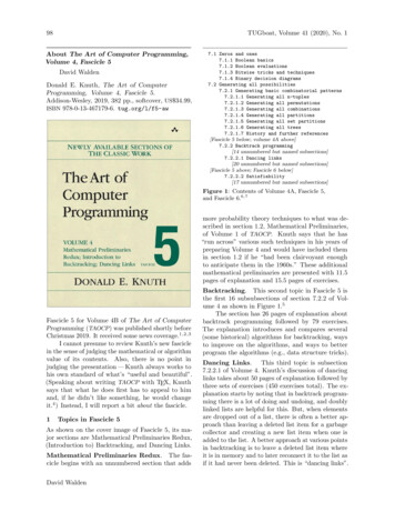
1BIntroduction to TINAObjectiveThe objective of this exercise is to become familiar with the TINA electrical circuit simulationpackage in order to create simple schematics and perform basic simulations. TINA stands forToolkit for Interactive Network Analysis and is produced by DesignSoft. The differencesbetween US (ANSI) and Euro (DIN) schematic symbols, and 3D components will be examinedalong with the use of virtual instruments to make simulated measurements. Please note that theprecise look of the windows, menus and dialog boxes may be slightly different from that pictureddepending on the version of TINA that is being used. Regardless of appearance, the functionalityremains. A free version of TINA, known as TINA-TI, is available from the Texas Instrumentsweb site at https://www.ti.com/tool/TINA-TIProcedureAfter logging into the computer, open TINA. If a desktop shortcut is not available TINA may beaccessed via the Programs menu under the TINA menu item. You will be greeted with somethingsimilar to the screen shown in Figure 1B-1. Depending on the version, the precise look of theprogram may be a little different from that shown (TINA-TI). There are two toolbar stripsimmediately below the menus. The topmost toolbar contains the usual File Open, Save, andsimilar commands, along with buttons for text insertion, zoom level and the like. At the extremeright end of this strip is search box for electronic components. The lower strip is made up of a setof tabbed toolbars for electronic components, measurement instruments and other devices.Selecting a given tab (e.g., Basic, Meters, Semiconductors, etc.) shows the toolbar for that set ofitems.TINA’s schematic capture facility is object based, that is, you “draw” a circuit by selectingpredefined objects such as resistors and transistors, and drag them onto the workspace. They arethen wired together using the mouse. You can zoom into or out of the workspace using themouse or the zoom toolbar button.16Laboratory Manual for Computer Programming

Figure 1B-1TINA will draw schematics using one of three formats. The first style uses the ANSI (NorthAmerican) standard for schematic symbols. The second style uses the DIN (Euro) standard. Thefinal style is called "3D" where components look more like photographs of the actual component.Examples are shown in Figure 1B-2 using ANSI, DIN and 3D. You can set the preferred formatvia the View- Options menu item. More on this in a moment.Figure 1B-2Laboratory Manual for Computer Programming17

Generally, we do not use the 3D style for most work. It is, however, useful for newcomers as away of reinforcing and practicing use of the resistor color code, and for general packageidentification (such as the TO-92 transistor case pictured in Figure 1B-2). TINA will show theproper color sequence for resistors using either two or three significant digits along with a propertolerance band (i.e., four or five bands). A comparison is shown in Figure 1B-3.Figure 1B-3Along with the appropriate electronic parameters of a device, physical data regarding shape andpinout are required if a printed circuit board (PCB) will be created. For example, a particulardevice such as an operational amplifier may be available in several different package stylesincluding through-hole or surface mount variants. Our goal here is to become familiar withcapturing the schematic and performing simulations, such as verifying a laboratory exercise.Consequently, we shall not concern ourselves with the needs of PCB layout at this point.To illustrate the use and editing of components, select the Basic tab and drag a DC voltage source(third item) onto the workspace. It will show up with a default voltage value and label. Doubleclick the symbol. A dialog box will pop up next to it as shown in Figure 1B-4.Figure 1B-418Laboratory Manual for Computer Programming

From this dialog you can change a variety of attributes, the most important of which are thevoltage value and the label. Double clicking any component will bring up a settings dialog boxalthough the precise items contained within it will vary from component to component. Forexample, for a resistor there will be a resistance setting instead of a voltage setting. If you needto remove a component, simply select it and hit the Delete key.Electronic components can be placed into two broad categories; generic parts and more accurate"real world" models typically generated by the manufacturer of that part. This is particularly truewith complex components or devices. For example, Figure 1B-5 shows a pair of NPN transistors.The one labeled "!NPN" is a simple generic model. The lower, highlighted transistor references aspecific part number, in this case the 2N3904, a popular general purpose device.Figure 1B-5Double clicking the generic transistor opens up its settings dialog box. Initially, under Type, itwill say "NPN", referring to the generic. Next to this is a small box labeled with an ellipsis (.).Clicking on the ellipsis will open a second settings box, the Catalog Editor. From here, a specificmanufacturer's part can be selected from the scrolling list on the left. If need be, specificparameters can be altered in the list on the right.Laboratory Manual for Computer Programming19

Remember, whenever you see the small ellipsis box, clicking on it will open another settings boxso that you can specify further details.Editing the position and orientation of a component is straightforward. Once the item is selected(highlighted in red by default) it may be moved using either the mouse or the cursor keys. If youneed to move a group of components, the mouse may be used to select several items by clickingand then dragging the mouse over them. Every component within the selection box will behighlighted and will move as a group. Components may also be rotated and flipped. Thesecommands can be accessed from the main menu, however, it is handy to remember certainkeyboard shortcuts (such as Ctrl-R for rotate right, or clockwise). Also note that it is possible toselect the text labels of components and move or rotate them independently of the component.This can be handy if a label becomes obscured by a wire. To do so, make sure the component isnot selected (unhighlighted) and then click directly on the label. It can now be moved or rotated.Along with editing the components, you may also customize the look of the work space. Fromthe file menu, select Page Setup. This opens the dialog box shown in Figure 1B-6 and allows youto specify the sheet size for the schematic and related properties.Figure 1B-6Other attributes, such as whether or not to show the grid, component values, labels, and the likecan be selected from the View menu. This is shown in Figure 1B-7. Of particular importance isthe final item in this list, Options, which was mentioned earlier. Selecting Options brings up theEditor settings box shown in Figure 1B-8.20Laboratory Manual for Computer Programming

Figure 1B-7The Editor options include the aforementioned ANSI, DIN and 3D styles. It also includes the basefunction for AC (it is recommended this be set to sine). Further, you can adjust the color schemefor your workspace and a few other global parameters.Figure 1B-8Laboratory Manual for Computer Programming21

OK, let’s create a circuit and perform a simulation. If you have been experimenting, remove anycomponents on your workspace (select with the mouse and then press the Delete key). From theBasic components tab, select a DC voltage source, two resistors and an earth ground symbol. Weshall make a series loop of the three elements with the negative end of the power supply atground. One resistor will need to be rotated 90 degrees (one horizontal and one vertical). In orderto wire the items together, move the mouse to the end of one component you wish to wire. Theconnection ends are denoted with a small red x. When the mouse cursor is close, it will turn intoa pen shape. Simply click on the lead of the component and move the mouse to the desired leadof another component. While moving, TINA will draw a red line. Clicking on the secondcomponent will create a proper wire (by default, colored black). Wires are always drawn alongthe horizontal and vertical with 90 degree bends, not directly from point to point. This is theproper way to draw a schematic in the vast majority of cases.To delete a wire, click on it to select it. You will see a set of small “handles” on it. To removethe wire, simply hit the Delete key. Note that you can also move the wire with those handles ifdesired.Note that if you move a component, TINA will automatically move the wires along with it. Youdo not have to rewire it. If a component is later deleted, this will result in "dangling wires" whichalso should be deleted.Figure 1B-9Once the components are in place and wired, double-click each component to set their values asshown in Figure 1B-9. We shall then add two the two voltmeters (fifth item in the Basic tab).Please note that it is perfectly acceptable to change the component values immediately after22Laboratory Manual for Computer Programming

dragging them onto the work space; you don’t have to wait until they are wired together. It issuggested, though, that you decide upon a particular workflow and stick to it otherwise thechances of forgetting to change components from their default values increases.The circuit is now ready to perform a simulation.From the Analysis menu, select DC Analysis- Calculate nodal voltages. In a moment, the valuesof the voltages will be printed next to the voltmeters. Also, a small window will pop up. Withthis window, you can investigate particular node voltages or component voltages and currents.You will notice that the mouse cursor will have changed shape into a measurement probe. Youcan click on a node to see a voltage with respect to ground (a node is denoted with a small, solidblack circle on the wire where items connect, such as where a meter connects to a wire). Further,if you click on a component, the voltage across it and the current through it will be displayed inthe little pop up window. This is a nice interactive feature.TINA also has a wide variety of virtual instruments. These can be accessed via the T&M (Testand Measurement) menu. For example, Figure 1B-10 illustrates a virtual oscilloscope. This hasthe advantage of immediacy (assuming you’ve used an oscilloscope before), however, it is notthe ultimate way to perform a simulation. We will look at even more powerful and flexible waysof creating simulations in the next exercise.Figure 1B-10Laboratory Manual for Computer Programming23

For now, you may wish to delete this new instrument from the work space and then save theexisting schematic. Remember to always save to either your student account or to a USB drive.Never save directly to the hard drive in lab.There are three very good “every day” uses for TINA during your studies: First, it is a very handytool for verifying lab results. That is, you can recreate a lab circuit, simulate it, and compare thesimulation to both your theoretical calculations and lab measurements. Second, it is a handy toolfor checking homework if you get stuck on a problem. Third, it is convenient for the creation ofschematics, for example, for a lab report. An easy way to do this is to draw the circuit, capturethe screen image (Windows key Print Screen key copies it into the clipboard) and then paste theimage into your favorite image manipulation program. From there you can crop it, changecontrast, etc. as needed and then paste the modified image into your lab report.At this point you may wish to experiment a bit by rewiring the circuit or to try building newcircuits. As with any tool, continued practice will hone your skill. Once you are done and havesaved the file (the extension should be .TSC), close TINA and then shut down the computer.24Laboratory Manual for Computer Programming

Laboratory Manual for Computer Programming25

2BMultisim ExtensionsObjectiveThe objective of this exercise is to become more familiar with the Multisim electrical circuitsimulation package in order to use more generalized simulations via the Grapher Window.ProcedureIn previous work we have examined the basic functionality of Multisim, namely basic schematiccapture functions such as component selection, placement, and parameter editing, along withsimple simulations using virtual instruments such as a Digital Multimeter (DMM) to measure DCvoltage. While virtual instruments are quick and easy to use, and offer some amount offamiliarity, they are necessarily limited in other aspects. Some of the issues with virtualinstruments include:1. Limited measurements per unit, for example a single measurement for a DMM, requiringmultiple units for multiple measurements.2. The need to rewire the instruments (and hence the schematic) in order to take differentreadings.3. Excessive amount of work space area obscured by the instrument(s) with accompanyingclutter.4. No convenient way of storing and recalling prior simulations.5. No convenient means of exporting simulated measurement data to other programs.To address these issues Multisim allows non-instrument simulations through the use of theGrapher window. The Grapher is a single,

tools and proceeds to the Python programming language. Python (version 3.X) was chosen for several reasons. First, it is a modern, open-source programming environment. Second, it has a relatively shallow learning curve meaning that new programming students can get up and running fair