Transcription
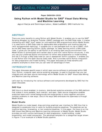
Paper SAS4384-2020Using Python with Model Studio for SAS Visual Data Miningand Machine LearningJagruti Kanjia and Dominique Latour, Jesse Luebbert, SAS Institute Inc.ABSTRACTThere are many benefits to using Python with Model Studio. It enables you to use the SAS Scripting Wrapper for Analytics Transfer (SWAT) package with the SAS Code node. It makesinteracting with SAS Viya easier for nontraditional SAS programmers within Model Studio.It is used within a SAS Code node for deployable data preparation and machine learning(with autogenerated reporting). It enables you to use packages built on top of SWAT, suchas the SAS Deep Learning Python (DLPy) package, for deep learning within a SAS Codenode. It gives you the ability to call Python in an existing open source environment fromModel Studio to authenticate and transfer data to and from native Python structures. It letsyou use your preferred Python environment for either data preparation or model buildingand call it through a SAS Code node for use or assessment within a pipeline. It enables youto use Python with the Open Source Code node. And it provides native Python integrationfor data preparation and model building. This paper discusses all these benefits andpresents examples to show how you can take full advantage of them.INTRODUCTIONThe paper discusses specific ways in which open source software is embraced within SASViya. Python, a popular open source scripting language, is used to illustrate how you canintegrate and use open source technology within Model Studio for SAS Visual Data Miningand Machine Learning software.Let’s start by introducing the various software and components developed by SAS that thepaper discusses.SAS ViyaSAS Viya is a cloud-enabled, in-memory, distributed analytics extension of the SAS platformthat makes it more scalable, fault-tolerant, and open. Open source integration enablesanalytical teams with varied backgrounds and experiences to come together and solvecomplex problems in new ways. One of the ways SAS embraces this openness is throughModel Studio.Model StudioModel Studio is a node-based, drag-and-drop graphical user interface for SAS Viya that isdesigned to accelerate time to value for building analytics pipelines. The pipelines can bemachine learning, forecasting, or text analytics pipelines. In this paper, the focus is on theSAS Visual Data Mining and Machine Learning component of Model Studio. Model Studioprovides you with various techniques for data preparation, model building, modelensembling, and model comparison. The advanced template for a categorical target shownin Figure 1 is an example of a Model Studio pipeline.1
Figure 1. Example of a Model Studio PipelineModel Studio is also designed to be extensible through nodes that are available in theMiscellaneous node category. The paper focuses on two of those nodes: the SAS Code nodeand the Open Source Code node.SAS Code Node and Open Source Code NodeYou can use the SAS Code node within Model Studio for data preparation and modelbuilding. This node enables you to add custom functionality to the software. Thisfunctionality can be traditional SAS code and procedures, SAS Viya procedures that callSAS Cloud Analytic Services (CAS) actions, or even open source code. You can use theSWAT package within the SAS Code node. The Open Source Code node is a Miscellaneousnode that can run Python or R code. The node can also be treated as a Supervised Learningnode so that your Python or R model can be assessed and compared with other ModelStudio models.SWATSAS Scripting Wrapper for Analytics Transfer (SWAT) is an open source Python package thatmakes it easy for programmers who are familiar with Python syntax to use the distributed,in-memory code base of SAS Viya and CAS for Python 2.7.x or 3.4 and later.USING PYTHON IN THE OPEN SOURCE CODE NODEThe Open Source Code node can execute Python or R scripts that are on the same machineas the compute server for SAS Viya in order to do data visualization, data preparation, ormodel building. This paper focuses on Python scripts.DATA PREPARATION USING PYTHON IN AN OPEN SOURCE CODE NODEIt is possible to do data preparation by using native Python syntax and have the output dataframe from the script be passed on to subsequent nodes. However, this is not something2
that can be deployed; it is designed for prototyping various feature engineering techniques.In order to pass the output data to the next node, you need to select the Use output datain child nodes property. The following Python code shows how to create a new feature,MORTPAID (the amount of the mortgage paid), simply by subtracting the value of themortgage due (MORTDUE) from the total mortgage value (VALUE), using PandasDataFrames that subsequent nodes will use.The dm inputdf and dm scoreddf data items are set by the Model Studio environment andcorrespond to Pandas DataFrames for the sampled input data and scored input data,respectively. You can find a complete list of generated data items in the Appendix.# Create a new variable to use in Pythondm inputdf['MORTPAID'] dm inputdf['VALUE'] - dm inputdf['MORTDUE']# Point output data name to modified data setdm scoreddf dm inputdfMODEL BUILDING USING PYTHON IN AN OPEN SOURCE CODE NODEIt is possible to do open source modeling by using various open source packages. Onepopular package for supervised machine learning is LightGBM. “Light” refers to its highspeed; GBM stands for gradient boosting machine, the algorithm that this method uses. TheLightGBM Python package is a gradient boosting framework that uses a tree-based learningalgorithm. LightGBM grows trees vertically, whereas other boosting algorithms grow treeshorizontally; this means that LightGBM grows tree leafwise, and other algorithms grow treeslevelwise. It chooses the leaf with maximum delta loss to grow. A loss function is a measurethat quantifies how well the prediction model is able to predict the expected outcome. Whengrowing the same leaf, a leafwise algorithm can reduce more loss than a levelwise algorithmcan. Because of its high speed, LightGBM can also process large data tables while using lessmemory than other boosting algorithms.Invoking the LightGBM package is easy. What is difficult is finding a good set ofparameters—that is, parameter tuning. LightGBM supports more than 100 parameters.Table 1 lists some of the basic parameters that you can use to control this algorithm.Table 1. Basic Parameters Available in LightGBM AlgorithmLightGBM ParameterDescriptionbagging fractionSpecifies the fraction of data to be used foreach iteration. This parameter is generallyused to speed up the training and avoidoverfitting.bagging freqSpecifies the frequency of bagging. Thevalue of 0 disables bagging; the valueindicates to perform bagging at every kthiteration.boosting typeSpecifies the type of algorithm that youwant to run. The gbdt is a traditionalgradient boosting decision tree algorithm.Other supported values are rf orrandom forest (random forest), dart(dropouts in multiple additive regressiontree), and goss (gradient-based one-sidesampling).3
LightGBM ParameterDescriptionfeature fractionSpecifies the percentage of featuresrandomly selected at each iteration ofbuilding trees. This parameter is usedwhen the boosting type is set to randomforest. For example, a 0.75 feature fractionmeans that LightGBM selects 75% of theparameters randomly at each iteration.learning rateSpecifies the learning rate parameter. Thisvalue determines the impact of each treeon the final outcome. A GBM algorithmworks by starting with an initial estimatethat gets updated using the output of eachtree. The learning parameter controls themagnitude of this change in the estimates.Typical values: 0.1, 0.001, 0.003, etc.metricSpecifies the metric to be evaluated in theevaluation set, such as gamma, area underthe curve, binary log-loss, or binary errormin data per groupSpecifies the minimal amount of data percategorical group. The default is 100.num iterationsSpecifies the number of boosting iterationsnum leavesSpecifies the number of leaves in one tree.The default is 31.objective or objective typeSpecifies the application of the model,whether it is a regression problem orclassification problem. By default,LightGBM treats the model as a regressionmodel. This is probably the most importantparameter. Specify the value of binary forbinary classification.In order to use the LightGBM package, you must first convert the training and validationdata into LightGBM data sets. After creating the lgb train and lgb valid data sets, a Pythondictionary is created that contains a set of parameters and associated values. Because thisis a classification problem, “binary” is used as the objective type and “binary logloss” as themetric. The boosting type is set to “gbdt” since you are implementing the gradient boostingalgorithm. The following methods are used to produce some results: plot importance plots the model feature importance.plot tree plots a specified tree.plot split value histogram generates a split-value histogram for the specifiedfeature of the model.Now let’s look at an example of how you can use this algorithm in the Open Source Codenode. The new pipeline shown in Figure 2 is created in a Model Studio project. The OpenSource Code node is preceded by an Imputation node to handle the missing values thatoccur in some of the variables.4
Figure 2. Model Studio Pipeline with Imputation Node and Open Source Code NodeIn the Open Source Code node, you enter the following code in the Code editor. The codetakes advantage of data items that are set by the Model Studio environment to integratethe Open Source Code node with the pipeline. The dm inputdf data item identifies the inputPandas DataFrame, whereas the dm partitionvar and dm partition train val data itemsidentify the partition variable and partition value, respectively, that correspond to thetraining observations. Model Studio supports a single partition variable whose valuesidentify the training, validation, and test observations, so you need to create light GBMtraining and validation data sets. Note that currently the Open Source Code node does notcreate data items for validation or test observations. When Model Studio generates apartition variable, the values 1, 0, and 2 are assigned to the observations of the training,validation, and test partitions, respectively. This is why the following code uses theexpression dm inputdf[dm partitionvar] 0 to produce the validation data set:import lightgbm as lgbimport osimport sysimport matplotlib as mplif os.environ.get('DISPLAY','') '':print('no display found. Using noninteractive Agg back end')mpl.use('Agg')import matplotlib.pyplot as plt# Make sure nominals are categorydtypes dm inputdf.dtypesnominals dtypes[dtypes 'object'].keys().tolist()5
for col in nominals:dm inputdf[col] dm inputdf[col].astype('category')# Training settrain dm inputdf[dm inputdf[dm partitionvar] dm partition train val]X train train.loc[:,dm input]y train train[dm dec target]lgb train lgb.Dataset(X train, y train, free raw data False)# Validation set for early stopping (optional)valid dm inputdf[dm inputdf[dm partitionvar] 0]X valid valid.loc[:,dm input]y valid valid[dm dec target]lgb valid lgb.Dataset(X valid, y valid, free raw data False)# LightGBM parametersparams {'num iterations': 60,'boosting type': 'gbdt','objective': 'binary','metric': 'binary logloss','num leaves': 75,'learning rate': 0.05,'feature fraction': 0.75,'bagging fraction': 0.75,'bagging freq': 0,'min data per group': 10}evals result {}# to record eval results for plotting# Fit LightGBM model to training datagbm lgb.train(params,lgb train,valid sets [lgb valid, lgb train],valid names ['valid','train'],early stopping rounds 5,evals result evals result)ax lgb.plot tree(gbm, tree index 53, figsize (25, 15),show info ['split gain'])plt.savefig(dm nodedir '/rpt tree.png', dpi 500)print('Plotting feature importances.')ax lgb.plot importance(gbm, max num features 10)plt.savefig(dm nodedir '/rpt importance.png', pad inches 0.1)print('Plotting split-value histogram.')ax lgb.plot split value histogram(gbm, feature 'IMP CLNO', bins 'auto')plt.savefig(dm nodedir '/rpt hist1.png')# Generate predictions and create new columns for Model Studiotmp gbm.predict(dm inputdf.loc[:,dm input])dm scoreddf pd.DataFrame()dm scoreddf[dm predictionvar[1]] tmpdm scoreddf[dm predictionvar[0]] 1 - tmp6
After you save the code, the pipeline is run. The Open Source Code node executes Pythoncode in the Python environment that is installed on the compute server where SAS Viya isrunning. The Node tab in Figure 3 displays the generated plot: the specified tree, the modelfeature importance plot, and the split-value histogram for the imputed variable CLNO.In its Results window, the Open Source Code node can display plots, tables, and files thatthe Python code generates, provided that those files are created in the node directory,which is specified by the dm nodedir data item. The files must have the rpt prefix and oneof the following extensions: .jpg (plots and images), .csv (tables), or .txt (text files).Figure 3. Open Source Code Node ResultsThe assessment results are calculated from the scored sampled project table thatcorresponds to the dm scoreddf data item. The Assessment tab in Figure 4 displays theassessment reports: lift reports, ROC reports, fit statistics table, and event classificationchart. The fit statistics table shows that the misclassification rate is 0.0274 for the trainingpartition, 0.0928 for the validation partition, and 0.0923 for the test partition.7
Figure 4. Open Source Code Node Assessment ResultsUSING SWAT IN THE SAS CODE NODEBecause you can use the SWAT package in a SAS Code node, a user familiar with Pythonprogramming can extend the functionality of Model Studio. You can use the Base SAS JavaObject to execute a Python script. Of note, a model that is written using SWAT can bedeployable, given that it generates either DATA step (DS1) score code or a SAS analyticstore (astore). Now let’s look at some examples of how you can produce deployable assetsfor both data preparation and model building.DEPLOYABLE DATA PREPARATION USING SWAT IN A SAS CODE NODEYou can execute the following code in a SAS Code node as a data mining preprocessingnode—that is, as an Unsupervised Learning node. The dmcas varmacro macro is used hereto generate a comma-separated list of categorical variable names enclosed in singlequotation marks./* Create additional variable lists */%dmcas varmacro(name dm class input, metadata &dm metadata,where %nrbquote(level in ('NOMINAL','ORDINAL','BINARY') and role 'INPUT'),key NAME, quote Y, singlequote Y, comma Y, append Y);Then you create a Python script as follows that invokes the CAS transform action to performa moment transformation of all the categorical variables. The CAS session macro variablesthat Model Studio initializes (dm cashost, dm casport, and dm cassessionid) are used to8
connect to the CAS session that is started when the SAS Code node runs. Thedm rstoretable macro variable identifies the SAS analytic store that can be used to score atable to generate the transformed variables./* Create Python script with SAS macro variables inserted */proc cas;file codef "&dm nodedir&dm dsep.dm srcfile.py";print "import swat";print "s swat.CAS(hostname '&dm cashost', port '&dm casport',session '&dm cassessionid')";print "s.transform(table dict(caslib '&dm caslib', name '&dm memname',where '&dm partitionvar &dm partition train val'),requestPackages dict(function dict(name 'TE', inputs [%dm class input],targets '&dm dec vvntarget', event '&dm dec event',targetsinheritformats True, inputsinheritformats True,mapInterval dict(method 'moments', args dict(includeMissingLevel True,nMoments 1)))), savestate dict(caslib '&dm caslib', name '&dm rstoretable',replace True))";run;Next, you pass the Python executable file that you created earlier to the Java classSASJavaExec by using the Base SAS Java Object. SASJavaExec runs the Python script withits command line argument and passes any output or reports any errors back to the SASViya log. In the following DATA step, you initiate the Java Object by giving the class thonExec) and the Python script name. (Youcan find a description of the Java class SASJavaExec in the following white gration/blob/master/SAS Base OpenSrcIntegration/SAS Base OpenSrcIntegration.pdf.)/* Set class path */%dmcas setClasspath();/* Execute Python script */data null ;length rtn val 8;declare SASPythonExec","&dm nodedir&dm dsep.dm srcfile.py");j.callVoidMethod("setOutputFile","&dm nodedir&dm dsep&lang. output.txt");j.callIntMethod("executeProcess", rtn val);j.delete();call symput('javaobj rtnval', rtn val);run;The following code shows how you use the dm metadata macro variable that identifies thetable containing the variables and attributes to reject the input categorical variables thatwere transformed. The dm file deltacode macro variable identifies a file that contains thespecified metadata changes that successor nodes will use./* Reject original inputs (optional) */filename deltac "&dm file deltacode";data null ;file deltac;set &dm metadata;9
length codeline 500;if level in ('NOMINAL','ORDINAL','BINARY') and role 'INPUT' then do;codeline "if upcase(NAME) '"!!upcase(tranwrd(ktrim(NAME), "'","''"))!!"' then do;";put codeline;codeline "ROLE 'REJECTED';";put 3 codeline;put 'end;';output;end;run;filename deltac;DEPLOYABLE MODEL BUILDING USING SWAT IN A SAS CODE NODEYou can execute the following code in a SAS Code node that has been moved into theSupervised Learning lane of Model Studio. This code produces a gradient boosting treemodel by calling the gbtrain action of the decisionTree action set./* Create additional variable lists */%dmcas varmacro(name dm class var, metadata &dm metadata,where %nrbquote(level in ('NOMINAL','ORDINAL','BINARY') and role in('INPUT','TARGET')), key NAME, quote Y, singlequote Y, comma Y, append Y);%dmcas varmacro(name dm input, metadata &dm metadata,where %nrbquote(role 'INPUT'), key NAME, quote Y, singlequote Y, comma Y,append Y);* Create Python script with SAS macro variables inserted;proc cas;file codef "&dm nodedir&dm dsep.dm srcfile.py";print "import swat";print "s swat.CAS(hostname '&dm cashost', port '&dm casport',session '&dm cassessionid')";print "s.loadactionset('decisiontree')";print "s.gbtreetrain(table dict(caslib '&dm caslib', name '&dm memname',where '&dm partitionvar &dm partition train val'),target '&dm dec vvntarget', inputs [%dm input], nominals [%dm class var],savestate dict(caslib '&dm caslib', name '&dm rstoretable', replace True))";run;/* Set class path */%dmcas setClasspath();/* Execute Python script */data null ;length rtn val 8;declare SASPythonExec","&dm nodedir&dm dsep.dm srcfile.py");j.callVoidMethod("setOutputFile","&dm nodedir&dm dsep&lang. output.txt");j.callIntMethod("executeProcess", rtn val);j.delete();call symput('javaobj rtnval', rtn val);run;10
DEPLOYABLE MODEL BUILDING USING DLPy IN A SAS CODE NODESeveral Python packages that use SWAT are tailored to specific use cases. One extremelypopular use case is the SAS Deep Learning Python (DLPy) package. This package wasdesigned specifically to make programming deep learning models more approachable byusing friendly Keras-like APIs. Conveniently enough, this package can be used within a SASCode node as well.In this example, the SAS Code node is preceded by the Feature Machine node, which is adata mining preprocessing node that generates features that address one or moretransformation policies. The new features can be generated to fix data quality issues suchas high cardinality, high kurtosis, high skewness, low entropy, outliers, and missing values.The new pipeline shown in Figure 5 is created in a Model Studio project.Figure 5. Model Studio Pipeline with Feature Machine and SAS Code NodesThe following code is specified in the Training code editor of the SAS Code node. Two lists ofvariables are generated using the dmcas varmacro macro: one for categorical inputvariables and one for all inputs, interval and categorical. The DLPy package uses the SASViya deep neural network action set deepLearn to generate the model. When the node isrun, the dm srcfile.py file is executed in the Python environment installed on the computeserver that is running SAS Viya./* Create additional variable lists */%dmcas varmacro(name dm class var, metadata &dm metadata,where %nrbquote(level in ('NOMINAL','ORDINAL','BINARY') and role in('INPUT','TARGET')), key NAME, quote Y, singlequote Y, comma Y, append Y);%dmcas varmacro(name dm input, metadata &dm metadata, where %nrbquote(role 'INPUT'), key NAME, quote Y, singlequote Y, comma Y, append Y);11
/* Create Python file to execute */proc cas;file codef "&dm nodedir&dm dsep.dm srcfile.py";print "import swat";print "from dlpy import Model, Sequential";print "from dlpy.model import Optimizer, AdamSolver";print "from dlpy.layers import *";print "import pandas as pd";print "import os";print "import matplotlib";print "from matplotlib import pyplot as plt";print "plt.switch backend('agg')";print "s swat.CAS(hostname '&dm cashost', port '&dm casport',session '&dm cassessionid')";print "s.loadactionset('deeplearn')";print "s.setsessopt(caslib '&dm caslib')";print "model Sequential(s,model table s.CASTable('simple dnn classifier', replace True))";print "model.add(InputLayer(std 'STD'))";print "model.add(Dense(20, act 'relu'))";print "model.add(OutputLayer(act 'softmax', n 2, error 'entropy'))";print "model.fit(s.CASTable('&dm memname',where '&dm partitionvar &dm partition train val'),target '&dm dec vvntarget', inputs [%dm input], nominals [%dm class var],optimizer Optimizer(algorithm AdamSolver(learning rate 0.005,learning rate policy 'step',gamma 0.9,step size 5), mini batch size 4, seed 1234,max epochs 50))";In the following code, the Graphviz utility is used to create and save plots as image files.The directed acyclic graph (DAG) of the model network is displayed. The summary of modeltraining history was written to the output.txt file, which is displayed as Python output. Aplot is created to visualize the training history and saved in an image file.print "outF open('&dm nodedir/ output.txt', 'w')";print "summary model.print summary()";print "print(summary, sep ' ', end '\n\n', file outF, flush False)";print "history model.training history";print "print(history, sep ' ', end '\n\n', file outF, flush False)";print "n model.plot network()";print "from graphviz import Graph";print "g Graph(format 'png')";print "n.format 'png'";print "n.render('&dm nodedir&dm dsep.rpt network1.gv')";print "outF.close()";print "th model.plot training history(fig size (15,6))";print"th.get figure().savefig('&dm nodedir&dm dsep.rpt train hist.png')";The dlExportModel action from the Deep Neural action set is used as follows to create theanalytic store table named by the dm rstoretable macro variable. When the script finishesrunning, Model Studio uses this analytic store to score the entire training table so thatassessment results can be produced.print "s.dlExportModel(modeltable 'simple dnn classifier',initWeights 'simple dnn classifier weights', randomflip 'NONE',randomCrop 'NONE', randomMutation 'NONE', casout '&dm rstoretable')";run;12
/* Set class path */%dmcas setClasspath();/* Execute Python script */data null ;length rtn val 8;declare SASPythonExec","&dm nodedir&dm dsep.dm srcfile.py");j.callVoidMethod("setOutputFile","&dm nodedir&dm dsep&lang. output.txt");j.callIntMethod("executeProcess", rtn val);j.delete();call symput('javaobj rtnval', rtn val);run;%let source &dm nodedir&dm dsep.;/* Rename png file that was created using graphviz function */data null ;rc rename("&dm nodedir&dm dsep.rpt network1.gv.png","&dm nodedir&dm dsep.rpt network1 gv.png", "file");run;In contrast with the Open Source Code node, which automatically generates reports, youhave to use the dmcas report utility macro as follows to indicate which reports to display inaddition to the reports that Model Studio automatically generates:/* Create a report to display network plot */%dmcas report(file &dm nodedir&dm dsep.rpt network1 gv.png, reportType Image,description %nrbquote('Network Plot'), localize N);/* Create a report to display training history plot */%dmcas report(file &dm nodedir&dm dsep.rpt train hist.png, reportType Image,description %nrbquote('Tree Plot'), localize N);/* Create a report to display Python output file */%dmcas report(file &dm nodedir&dm dsep. output.txt, reportType CodeEditor,type TEXT, description %nrbquote('Python Output'), localize N);The results of the SAS Code node are displayed in Figure 6. This includes the submitted SASCode, an automatic report produced by Model Studio, and the three requested reports: twoimage files and the text file containing the Python output.13
Figure 6. SAS Code Node ResultsThe Assessment tab in Figure 7 displays the assessment reports: lift reports, ROC reports,fit statistics table, and event classification chart. The fit statistics table shows that themisclassification rate is 0.0903 for the training partition, 0.1079 for the validation partition,and 0.1040 for the test partition.Figure 7. SAS Code Assessment Results14
Model Studio supports a variety of model interpretability reports, such as partialdependence (PD) plots and individual conditional expectation (ICE) plots. Figure 8 shows allsupported global interpretability and local interpretability reports that you can create. Thepipeline is rerun to create these reports. The figure displays the surrogate model variableimportance table, PD plot, PD and ICE overlay plot, and LIME explanations plot on theModel Interpretability tab.Note that the generation of such reports is possible only because there is a representationof the model as score code; in this case it is an analytic store. If the model does notproduce score code but instead generates only a scored table, then the only modelinterpretability report that you can generate is the surrogate variable importance plot,because the other reports require rescoring.Figure 8. SAS Code Node Model Interpretability ResultsUSING PYTHON IN AN EXISTING OPEN SOURCE ENVIRONMENTFROM MODEL STUDIO TO AUTHENTICATE AND TRANSFER DATATO AND FROM NATIVE PYTHON STRUCTURESAs explained earlier, the Open Source Code node executes Python scripts that are on thesame machine as the compute server where SAS Viya is running. However, you can submitPython scripts on a remote server by using the remrunner and Paramiko packages.The remrunner (remote runner) package enables you to transfer a local script file to aremote host and execute it. The named file is copied to a temporary location on a remotehost, its permissions are set to 0700, and the script is then executed. During cleanup, the15
[PID] directory and all its contents are removed before the connections are closed. Theremrunner package uses the Paramiko package for SSHv2 protocol implementation. Thecurrent limitation of the remrunner package is that it assumes that SSH keys, which allowpassword-free log-ins, are already in place. There is no option to prompt for a password orSSH passphrase.In this example, the SAS Code node is used to create and submit a Python file to a remotesystem and transfer some of the results back to the system where SAS Viya is running. TheFeature Machine node is used to generate new features by performing variabletransformations to improve data quality and model accuracy.The SAS Code node is again used as the Supervised Learning node. However, this time itcreates and submits a Python file to a remote system and displays results from executingthe Python model. This differs from the previous examples that use the Open Source Codenode, where a sample of the data was downloaded to the SAS Viya client and thenconverted to a Pandas DataFrame. Here SWAT is used to directly access the training tableloaded into CAS and to create a DataFrame from the entire table. Then the scored table thatis produced by an XGB Classifier Python model is uploaded into the CAS session so thatModel Studio can assess the entire score table for this Python-generated model.The new pipeline shown in Figure 9 is created in Model Studio.Figure 9. Model Studio Pipeline with Feature Machine and SAS Code NodesYou can find the complete code that is specified in the SAS Code node editor in GitHub atthe following link: -2020/tree/master/papers/4384-2020-KanjiaAs before, you start by creating two variable lists: one for categorical input variables, andthe other for all inputs, interval and categorical.16
* Create additional variable lists;%dmcas varmacro(name dm class var, metadata &dm metadata,where %nrbquote(level in ('NOMINAL','ORDINAL','BINARY') and role in('INPUT','TARGET')), key NAME, quote Y, singlequote Y, comma Y, append Y);%dmcas varmacro(name dm input, metadata &dm metadata, where %nrbquote(role 'INPUT'), key NAME, quote Y, singlequote Y, comma Y, append Y);Then you use the first CAS procedure step to create a Python file named gb01.py, whichwhen executed runs an XGB classifier algorithm. This algorithm is an implementation ofgradient boosting decision trees designed for speed and performance.proc cas;file codef "&dm nodedir&dm dsep.gb01.py";print "#!/usr/bin/python";print "import os";print "import paramiko";print "import pandas as pd";print "import swat, sys";print "from sklearn import ensemble";print "from xgboost import XGBClassifier";print "from xgboos
Using Python with Model Studio for SAS Visual Data Mining and Machine Learning Jagruti Kanjia and Dominique Latour, Jesse Luebbert, SAS Institute Inc. ABSTRACT There are many benefits to using Python with Model Studio. It enables you to use the SAS Scripting Wrapper for Analytics Transfer (SWAT)