WIXLIB

7We proceed as follows: Section 2 (Predictive Modeling with an Example) introduces predictive modeling with a mortality predictionexample. Using U.S. county level data including mortality, demographic and economic information, thissection shows a subset of tools and models used in predictive analytics but provides a comprehensiveoverview of a typical predictive modeling process including data processing, model choice, model training,model validation, result communication and model implementation. Readers will be able to understand thekind of problems that predictive modeling can help solve, different tools and models that are available toperform the analysis, and ways to assess model accuracy and address important issues such as overfitting.Section 3 (Literature Review) discusses the areas that predictive modeling may be applied to improve thepension industry. It includes both existing and potentially future applications and research. This helpsreaders better understand the potential impact of predictive analytics on pension and retirement in thefuture.Section 4 (Case Study: De-risking Activity Prediction) uses Form 5500 data published by the U.S.Department of Labor and studies the demographic profile, fund contribution, asset allocation, fundingstatus, demographic profile, and actuarial assumptions using plan level data to identify useful data, trend,and patterns for pension plan management. It builds a prediction system to identify plans that may haverisk transfer activities in the near future. Supervised learning is applied with a detailed explanation of datapreparation, model training, model validation, and model selection.Section 5 (Conclusion) summarizes the key points of this research and concludes the main body of thereport.Appendix A (Predictive Modeling in Condensed Form) provides a comprehensive overview of predictivemodeling. We encourage interested and advanced readers to review the Appendix. We have deliberatelydesigned Appendix A to mirror the body of the report but with more details and examples. Therefore,topics can be read at a high-level in the body of the report and further explored in the parallel area of theAppendix.Appendix B (Open-Source Python Program) describes the Python programs built for this research that arepublicly accessible.Copyright 2021 Society of Actuaries Research Institute

8Section 2: Predictive Modeling with an ExampleUsing a simple yet relevant topic as an example, this section introduces some of the basic elements of a predictiveanalytical task including data, model selection, and prediction. Discussions of modeling choices are avoided in thissection but covered in Appendix A, to make this section as light as possible. The idea here is not to get obsessedwith all the details but to understand the process and core concepts so that other problems can be approached inthe same mechanical and systematic way.Geolocation has been widely used in insurance pricing for a long time, such as life products that protect againstdeath events, and non-life insurance products like auto insurance. For the pension industry, geolocation of planparticipants can help evaluate the aggregate mortality rate of a pension plan. It may also be beneficial for individualretirement planning, recognizing that other factors such as age and health conditions may have a bigger impact onmortality. In this example, we try to predict the U.S. county level mortality rate compared to the national averagemortality rate.Two datasets are used in the relative mortality example: United States Mortality Rates by County 1980-2014 by Global Health Data Exchange3. It provides mortalityrates of 3,142 counties due to 21 mutually exclusive causes of death.2016 Planning Database by U.S. Census Bureau4. It provides information about urbanization, gender, age,race distribution, education level, health insurance, and household incomes for each county.Table 1 lists the final variables used in this example. The response variable “MR Relative” which we want to predictis defined as the county level mortality rate divided by the national average mortality rate. The explanatory variablesthat are used to explain the response variable contain some high-level demographic and economic information.Some of the explanatory variables are created based on the original dataset to better represent the information wewant to use for this analysis.3Institute for Health Metrics and Evaluation (IHME). United States Mortality Rates by County 1980-2014. Seattle,United States: Institute for Health Metrics and Evaluation (IHME), nited-states-mortality-rates-county-1980-20144The U.S. Census Bureau, 2017. “2016 Planning ight 2021 Society of Actuaries Research Institute

9Table 1RELATIVE MORTALITY DATASET VARIABLESVariableNoteTypeMR RelativeRelative mortality multipleResponseland per capitaLand area (sq.mi.) per personExplanatoryurbanized pop pctPerc. of population living in Area defined as an UrbanizedArea (50,000 or greater)Perc. of population living in Area defined as an UrbanCluster Area (2,500-49,999)Perc. of population living in Area outside of an UrbanArea or Urban ClusterExplanatorymale pctPerc. of male residentsExplanatoryfemale pctPerc. of female residentsExplanatoryage 5 pctPerc. of age below 5Explanatoryage 5 17 pctPerc. of age 5-17Explanatoryage 18 24 pctPerc. of age 18-24Explanatoryage 25 44 pctPerc. of age 25-44Explanatoryage 45 64 pctPerc. of age 45-64Explanatoryage 65 pctPerc. of age 65 and overExplanatoryhispanic pctPerc. of Hispanic origin populationExplanatorywhite pctPerc. of White populationExplanatoryblack pctPerc. of Black and Africa American populationExplanatoryaian pctPerc. of American Indian and Alaska Native populationExplanatoryasian pctPerc. of Asian populationExplanatorynhopi pctPerc. of Native Hawaiian and Other Pacific IslanderpopulationPerc. of some other race populationExplanatorynot hs pctPerc. of people 25 years old and over who are not highschool graduatesExplanatorycollege pctPerc. of persons 25 with Bachelor's degree orhigherPerc. of people classified as below the poverty levelExplanatoryExplanatoryno health ins pctPerc. of people with one type of health insurancecoveragePerc. of people with two or more types of healthinsurance coveragePerc. of people with no health insurance coveragemed hh incMedian household incomeExplanatoryavg hh incAverage household incomeExplanatorymed house valueMedian house valueExplanatoryavg house valueAverage house valueExplanatorystate avgAverage relative mortality at state levelExplanatoryurban cluster pctrural pop pctsor pctpoverty pctone health ins pcttwo plus health ins lanatoryExplanatoryOne question to answer before performing the analysis is why do we need to predict the relative mortality multipleCopyright 2021 Society of Actuaries Research Institute

10in the first place? If the county level relative mortality multiple is already known, it can simply be applied to adjustthe mortality assumption at the county level. For applications in the pension field, the relationship found at thecounty level can be applied at a more granular level such as to zip codes. For instance, say we know the relativemortality for Westchester County in New York. There are numerous zip codes within Westchester County. Mortalitydata is not publicly available at the zip code level. We can, however, collect explanatory variables at the zip codelevel and then map those to a representative county or set of counties. If we know the relative mortality of thecount(ies) we can then use this as a proxy for the relative mortality at the more detailed zip code level.Figure 1 shows a typical predictive modeling process, which is composed of two major parts: calibration andimplementation.Figure 2PREDICTIVE MODELING SAMPLE PROCESSData ExplorationData CleaningModel Validation Data Validation Feature Engineering Dimensionality Reduction Examine different model types Hyperparameters Error Function OverfittingCalibrationModel Training Descriptive Statistics Relationships Data Visualization Goodness-of-fit Measures Scatter Plots Feature ImportanceResult Communication Result Visualization Model SelectionModel Implementation Prediction Process Model UpdatingThe rest of this section explains each component in the process using the example of relative mortality prediction.2.1 EXPLORATORY DATA ANALYSISAs the first step in predictive modeling, exploratory data analysis (EDA) is a model-free approach to summarize dataand relationships among variables using descriptive statistics and visualization. The goal of EDA is to provide anoverview of the data and spot any interesting trends or relationships that may be helpful for constructing predictiveCopyright 2021 Society of Actuaries Research Institute

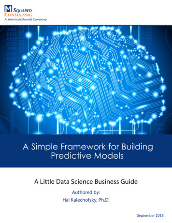
11models and validating the results. Pension actuaries already employ a version of EDA in their standard valuationactuarial reports when they plot metrics such as trends in funded status and population statistics.Descriptive statistics, correlation, and data visualization are typical tools used during EDA to find prominent andsimple patterns. Table 2 shows some descriptive statistics of the variables used as explained in Table 1.Table 2SAMPLE DESCRIPTIVE STATISTICSVariableMR 981.093rdQuartile1.22land per capita0.100.680.000.010.020.0426.04urbanized pop pcturban cluster pct30%21%35%21%0%0%0%4%6%16%61%34%100%100%rural pop pctmale pct49%50%29%2%0%45%26%49%46%49%69%50%100%72%female pct50%2%28%50%51%51%55%age 5 pctMeanMinMedianMax2.096%1%3%6%6%7%13%age 5 17 pct17%2%7%16%17%18%27%age 18 24 pct9%3%2%8%9%10%47%age 25 44 pct24%3%14%23%24%26%43%age 45 64 pct28%3%10%26%28%29%45%age 65 pct15%4%3%13%15%17%33%hispanic pct9%12%0%3%5%10%96%white pct76%17%3%68%80%89%99%black pct9%12%0%1%5%14%78%aian pct2%6%0%0%0%1%83%asian pct2%3%0%0%1%2%43%nhopi pct0%0%0%0%0%0%11%sor pct0%0%0%0%0%0%3%not hs pctcollege pctpoverty 0%54%44%one health ins pct66%6%36%63%67%70%84%two plus health ins 42,16314%47,78616%54,56461%132,203no health ins pctmed hh incavg hh inc63,25913,97130,08654,29460,70369,175152,424med house 4avg house 0.110.820.981.031.111.30state avgDescriptive statistics can also be represented as graphs to provide an overview of the data in a vivid way. Figure 2shows the degree of urbanization, age mix and health insurance coverage.Copyright 2021 Society of Actuaries Research Institute

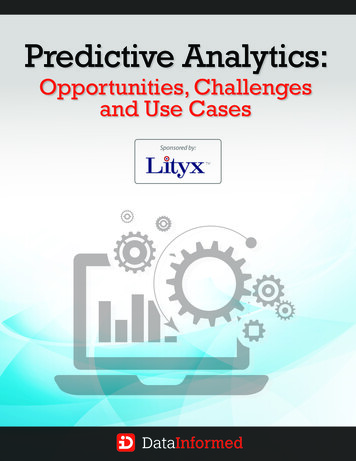
12Figure 2SAMPLE PIE CHARTSFigure 3 are the box plots that show the distributions of variables. Each box represents the data between the firstand third quartile (Q1 and Q3), with the line in the middle as the median. The box extends to wider data rangebetween [Q1 – 1.5(Q3 – Q1), Q3 1.5(Q3 – Q1)], where available. For outliers outside this range, they are plotted asindividual dots. It is clear that variables such as “land per capita”, “male pct”, “age 18 24 pct” and“med house value” are all right skewed.Figure 3SAMPLE BOX PLOTSDescriptive statistics are helpful for gaining a high-level understanding of the data. However, data can behavesignificantly differently with the same or similar descriptive statistics. Visualization is a powerful tool to further studythe details that may be missed in descriptive statistics. Figure 4 illustrates the relative mortality data on a map. ItCopyright 2021 Society of Actuaries Research Institute

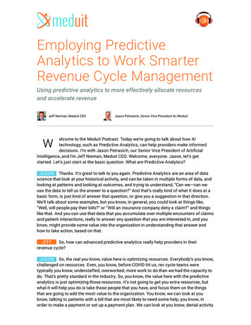
13can help us set some benchmark about areas where mortality rates are relatively higher compared to nationalaverage.Figure 4U.S. MORTALITY LEVEL BY COUNTYTo explore the relationship among variables, correlation matrices in the format of a heatmap can be used to quicklyidentify highly correlated pairs. Figure 5 shows the heatmap of some selected variables in the dataset. It is notablethat the response variable is negatively correlated with household income(“med hh inc”), housevalue(“med house value”), college education(“college pct”) and positively correlated to poverty(“poverty pct”).Some explanatory variables such as household income(“med hh inc”) and house value(“med house value”) arehighly correlated.Copyright 2021 Society of Actuaries Research Institute

14Figure 5SAMPLE HEATMAPEDA is a general concept that contains all kinds of data exploration without formal modeling. What is describedabove is only a small portion of what is available in this field5.5Two recent books on the subject include, “How Charts Lie: Getting Smarter about Visual Information” and “The Truthful Art: Data, Charts, and Maps forCommunication”. Both are by Alberto Cairo and are recommended for readers who are more interested in this area.Copyright 2021 Society of Actuaries Research Institute

152.2 DATA CLEANINGAfter the EDA, it is easier to define the prediction task and determine what data may be used. However, before thedata can be fed into the predictive models, additional processing is often needed to adjust the data inputs topotentially improve model accuracy. Missing data treatment, data normalization, feature engineering, anddimensionality reduction are often used in the data cleaning process. In this simple example, part of the first threecomponents is used.Missing data is quite common, especially with large datasets. In the census dataset where demographic andeconomic information is stored, 33 out of 3,142 counties do not have household income and house value data,which are correlated with relative mortality level. Normally a few choices are available to treat data records withmissing data. They can be removed, replaced with average value or value in a similar data record, or flagged in anindicator variable to represent that the data is missing. In this example, all 33 records are removed considering thatthe volume of the remaining data is still large enough for a meaningful analysis.When explanatory variables have different levels of magnitude, they may need to be normalized so that theparameter calibration will not be dominated by a small portion of the variables, and therefore better reflect therelationship between response variable and explanatory variables. As shown in T

Predictive analytics is statistical analysis aimed at making predictions about future or unobservable outcomes using data and techniques such as statistical modeling and machine learning. Actuaries have been working with predictive models such as linear regression and generalize