Transcription
Tree reduced ensemble clustering and distances between clustertrees based on a graph algebraic frameworkR.W. OldfordUniversity of WaterlooWaterloo, Ontario, CanadaW. ZhouUniversity of WaterlooWaterloo, Ontario, CanadaFebruary 20, 2014AbstractThe problem of finding multiple, possibly overlapping clusters is shown to share mathematical structure with the problem of combining the outcomes from multiple clusterings. Both problems can be cast interms of sets of graphs, which we call graph families. A graph algebraic framework is developed throughillustrative examples and formally presented. By way of this framework, a new multi-clustering methodwe call tree reduced ensemble clustering is developed that is applicable to the outcomes of any combination of clustering methods. Several examples including k means, model-based clustering, single-linkageand complete-linkage clustering are used to illustrate and to develop the graph algebraic framework forclustering and multi-clustering. A new distance between cluster trees is presented and shown to be usefulin the comparative study of clustering outcomes.Keywords: cluster trees, graph families, ensemble clustering, multi-clustering, partitions, hierarchicalclustering, graph-based clustering, consensus clustering, distance between cluster trees1IntroductionIn this paper we develop a new ensemble method for combining multiple clustering outcomes. The method isagnostic about the source of the clusterings and so is not tied to any clustering method such as k-means. Theensemble method, TREC, or tree reduced ensemble clustering, produces a single cluster tree as its output.The result is not a dendrogram as would be produced by a typical hierarchical clustering method like singlelinkage, but rather a cluster tree similar in structure to the density cluster trees described in (Hartigan 1985)though requiring no such density interpretation.To develop the methodology, we cast the multiple clustering problem as one of summarizing the clusterstructure provided by a set of graphs on the same vertex set. We call a set of such graphs a graph family andintroduce some formal mathematical structure that describes the operations performed on a graph family toproduce a cluster tree.The methodology is developed via simple examples and then applied on data where clustering outcomescan be from partition methods like k-means and Gaussian mixture model based clustering, hierarchicalmethods like single and complete linkage, or any mixture of partition and hierarchical methods. The outcomesneed not even be generated by any formal method or algorithm whatsoever. Two data sets, one generatedfrom a mixture of three Gaussians and the other an artificial pair of spirals are clustered by the variousmethods to motivate and to illustrate the methodology.The methodology used to produce the ensemble method is then formalized mathematically and thenature of the various operations briefly described. More importantly, these operations, their mathematicalcharacteristics, and the sets on which they operate together form a graph algebraic framework in whichthe problem of multiple clustering may be cast. Various sets of graph families can be placed within theframework and connected to isomorphic spaces of matrices and of cluster trees. The TREC methodology isseen to provide a means of projecting the outcome (or outcomes) of any clustering method into a space of1
cluster trees. Moreover, a metric is defined on a space of matrices which is isomorphic to the space of clustertrees. This induces a corresponding metric on the cluster trees which can be used to compare the the clustertrees and hence the characteristics of the clustering methods which led to them.The paper separates into two major parts. The first is Section 2 where the proposed methodology isdeveloped via illustrative examples. Relevant literature review is used to motivate the approach. Oncedeveloped, the methodology is applied to the example data sets. These examples show how the TRECmethodology works. The second major part is Section 3 where the formal graph algebraic framework ismathematically abstracted and summarized. All necessary proofs can be found in the Appendix. In Section3 the distance measure is also introduced and applied to the cluster trees constructed in Section 2.4 for theGaussian mixture data. These distances are used in multidimensional scaling to position the various clustertrees in a two dimensional space. This provides a quick visual means to assess various characteristics of theresulting cluster trees (TREC performs well).The paper ends with some brief concluding remarks and future directions in Section 4.2Developing the methodologyIn this section we develop our methodology through the exploration of several examples.Section 2.1 considers the problem of multiple clusterings and how others have proposed to address it.This review suggests that a weighted adjacency matrix, Aω , plays an essential role in these solutions andhence that a graph-theoretic approach could be a helpful underpinning to any such investigation.In Section 2.2, we examine the value of using this matrix by applying it to multiple clustering of agenerated data set where the underlying true cluster structure is known (a Gaussian mixture and usingoutcomes from different k-means clustering outcomes). This examination, however, indicates that the rawAω has shortcomings as a cluster summary.To overcome these, in Section 2.3 the problem of multiple clustering is cast in terms of families of graphs(each graph representing a clustering). The goal becomes to transform the graph family so that its resultingweighted adjacency matrix, Aρ , is a more useful summary of the multiple clusterings. Working throughsimple examples, Section 2.3 develops and illustrates the sequence of transformations. This sequence definesthe ensemble method we call tree reduced ensemble clustering, or TREC.In Section 2.4 TREC is illustrated by applying the method to several examples. In addition to theseveral outputs from k-means considered earlier, in this section we also combine the output from severalother clustering methods including Gaussian mixture model clustering, and simple and complete linkage.The method applies universally to the outcome of all methods which produce one or more clusterings.2.1Motivation – multiple clusteringsThe problem of multiple clusterings arises for many reasons. All hierarchical clustering methods inherentlyproduce multiple clusterings as a set of nested partitions (e.g. see Hartigan 1975). Other methods intentionally produce multiple non-nested clusterings to capture different facets of similarity between objects (anotable early example being ADCLUS, from the psychometric literature – Shepard and Arabie 1975, 1979).Different methods have often arisen from differing philosophies or views as to the purpose of the clustering.These include, for example, teasing apart different notions of humanly perceived similarity between stimuli(e.g. Tversky 1977; Shepard and Arabie 1979), fitting mixture distributions to sample measurements (e.g.Fraley and Raftery 1999), optimizing an objective function designed to capture “natural” spatial structurein dimensional data (e.g. k-means, MacQueen 1967), determining high density modes from a sample (e.g.Hartigan 1981; Ester et al. 1996; Stuetzle 2003), and determining approximate graph components in a similarity graph (e.g. Donath and Hoffman 1973; Meila and Shi 2001), to mention the more common approaches.Multiple clusterings can also arise from multiple local optima (e.g. k-means, MacQueen 1967) or simply frommultiple values of some “tuning parameter” (e.g. again k-means, Ashlock et al. 2005). Sometimes multipleclusterings are even induced by resampling (e.g. Topchy et al. 2004) so that they can be later combined.Finally, in practice one might routinely choose a variety of methods, knowing in advance that each was2
sensitive to a different kind of cluster structure (e.g. k-means and complete linkage prefer globular clusterswhile single-linkage will favour stringy clusters), so as to cover a wide range of possibilities.Multiple clusterings might be summarized by a single partition (e.g. as in Strehl and Ghosh 2002;Dimitriadou et al. 2001), by a single tree (as does every hierarchical clustering or more recently as doesFred and Jain 2002), or even by several trees as in Carroll and Corter (1995). The multiple clusteringsthemselves could be used to produce a new similarity matrix which is then itself used as input to someclustering algorithm, yielding whatever is the natural output of that method and begging the question asto which algorithm it would be best to use (e.g. Fred and Jain 2002; Ashlock et al. 2005; Strehl and Ghosh2002) – curiously, one clustering algorithm might be recommended to produce multiple clusterings and adifferent one for their combination (e.g. Fred 2001; Fred and Jain 2002; Ashlock et al. 2005). Alternatively,the cluster ensemble problem could be cast as another optimization problem whereby a final partition wouldbe chosen to maximize some criterion, like a normalized mutual information measure (e.g. Strehl and Ghosh2002), involving the given collection of clusterings. Either way, a multiple clustering is replaced with a singleclustering problem which has access to the similarity information accumulated across the original clusterings.In what follows, we take a somewhat different approach. We begin with a set G of m graphs Gk andtheir corresponding adjacency matrices Ak ,Pfor k 1, 2, . . . , m. We might reasonably summarize this set bymthe sum of these adjacency matrices AG k 1 Ak . Perhaps not surprisingly, this simple sum is related toa popular means of summarizing cluster ensembles.To see this, first consider how ADCLUS (Shepard and Arabie 1975, 1979) constructs multiple, possiblyoverlapping clusters. The approach is based on approximating an original similarity matrix, S [s ij ], witha new one, S [sij ], constrained to have the following structure:sij KXwk pik pjk .k 1Here, K is the total number of (possibly overlapping) clusters, wk weights the importance (or “psychologicalsalience” as in Shepard and Arabie 1979) of cluster k and pik is 1 if i appears in cluster k and 0 otherwise.For n objects, the kth cluster corresponds to a binary vector pk (p1k , p2k , . . . , pnk )T . The ADCLUS derivedn n similarity matrix S [sij ] can also be written asS KXwk pk pTk P W P T(1)k 1where now W is a K K diagonal matrix of weights and P is the n K matrix whose kth column is pk .Note that, although there is no restriction on the diagonal terms of S in this representation, only the offdiagonal similarities are of interest in clustering.Multiple clusterings can use the same representation. For example, suppose we have r partitions ofn objects. Following Strehl and Ghosh (2002), the kth partition is represented as a binary membershipindicator matrix, P (k) having n rows and as many columns as there are clusters in that partition. Eachcolumn of P (k) is a binary vector representing a single cluster with 1 indicating membership in that cluster.A similarity matrix is constructed asS rXP (k) (P (k) )T P P T(2)k 1where P [P (1) , · · · , P (r) ]. This sum is equivalent to a voting mechanism where each cluster contributesone vote to every pair of objects within it. Subsequent clustering from this similarity matrix is the basis ofthe clustering ensemble methods used in Strehl and Ghosh (2002), Fred and Jain (2002), and Ashlock et al.(2005). Again, only the off-diagonal terms are of value.Each of the above equations can be re-expressed in terms of adjacency matrices Ak . For equation (1), wenote that pk pTk is a symmetric n n matrix whose off-diagonal elements correspond to the adjacency matrix,3
Ak , of the graph on n nodes with edges only between all pairs in the kth cluster. Equation (1) becomesS KXwk pk pTk k 1KXwk Jk k 1KXw k Ak(3)k 1where Jk is a diagonal matrix, diagonal(pk ) formed from the elements of pk . Similarly, for equation (2),P (k) (P (k) )T is a symmetric n n matrix whose off-diagonal elements correspond to the adjacency matrix ofthe graph on n nodes having complete graph components for each cluster in the kth partition. Equation (2)becomesrrrXXXS P (k) (P (k) )T Jk Ak(4)k 1k 1k 1where again Jk is a diagonal matrix, but now formed from the elements of kth partition with Jk diagonal(P (k) 1). If the partition matrix P (k) always includes a column for every singleton cluster in thepartition, then Jk is simply the n n identity matrix and equation (4) is simplyS rIn rXAk(5)k 1In all of these cases, the diagonal terms are of no import and we need only the matrix formed from a weightedsum of adjacency matrices. If we further restrict consideration to unity weights, then both equations (3) and(4) lead to a sum of adjacency matricesmXAk(6)k 1for appropriately defined m.2.2Using the raw weighted adjacency matrixThe previous section suggested that the sum of the adjacency matrices of equation (6) contains informationon the ensemble of the multiple clusterings. To assess this, we consider an example of multiple clusteringsproduced by different restarts of a k-means algorithm on data from a simple Gaussian mixture of knowncluster structure. While this investigation will show that this sum does contain considerable information onthe ensemble, it will also show that it also can provide highly variable detail that can hide important clusterstructure as well.2.2.1Data from a Gaussian mixtureFigure 1 shows a sample 300 points, 100 drawn from each of three distinct two dimensional Gaussians. Thecircles are drawn from the first Gaussian (Group 1 of Figure 1), the squares from the second (Group 2), andthe triangles from the third (Group 3). The first and second Gaussians are located closer to each other thaneither is to the third. The underlying hierarchy generating the groups is the tree of Figure 2.Suppose, as in Fred and Jain (2002) or Ashlock, Kim, and Guo (2005), we were to attempt to cluster thesedata using a partitioning algorithm like k-means. Clearly no hierarchical clustering could result. However,because k-means will only find local optima, random restarts of k-means will typically output differentclusterings (even with the same value of k). The ith restart will produce a partition, P (i) , and hence graphGi (having Pk complete components) with adjacency matrix Ai . With m random restarts, we compute themsum Aω i 1 Ai of these adjacency matrices and then examine Aω to uncover any consensus clusteringpattern.A simple visual means to display the sum Aω is as a pixel map, or pixmap. A pixmap can be used todisplay the contents of the matrix Aω by replacing each matrix element by a tiny square or pixel (i.e. a300 300 array of pixels in this case) whose colour saturation is determined by its corresponding value inthe total adjacency matrix, Aω – the larger is the value, the darker is the colour. Diagonal cells are assignedthe maximum saturation for display purposes.4
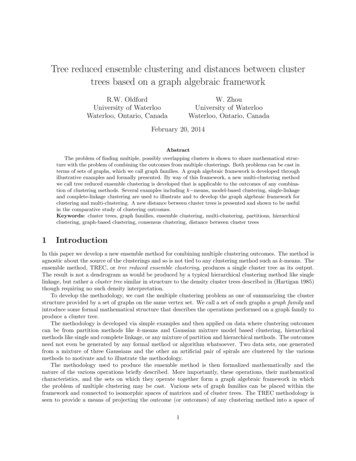
1077-50586-10Group 1: 1-100Group 2: 101-200Group 3: 201-300-10-50510Figure 1: A data set from a mix of Gaussians (points numbered 77 and 86 are identified)Groups 1, 2, and 3Groups 1 and 2Group 1Group 3Group 2Figure 2: The true hierarchical cluster tree generating the Gaussian data2.2.2Clusterings from k-means with k 3 and 10 random restartsThe sum of the adjacency matrices from 10 random restarts of k-means clustering (with k 3 each time)is shown as the pixmap of Figure 3(a) with rows (numbered 1 to 300 from the top) and columns (1 to 300from the left) matching the indices of the points from Figure 1. The more often a pair of points has beenassigned to the same cluster over the 10 restarts, the greater the saturation of colour in the correspondingcell.The three larger dark squares in Figure 3(a) correspond to the three groups of 100 points from Figure1 indicating that the different restarts have often placed each group’s points within its own cluster. Therestarts have also often placed points in group 1 in the same cluster as points from group 2 as shown by thelighter coloured off-diagonal squares where group 1 points are paired with group 2 points. This is becausegroups 1 and 2 are near each other and are elliptically shaped whereas k-means will often (depending onthe restart) mix the two groups to form its preferred circular clusters. This preference for circular clustersalso explains the two parallel lines (vertical and horizontal) corresponding to points 77 and 86 (see Figure1) which were assigned more often to the same cluster as points from group 2 than a cluster of points from5
(a) Rows and columns in original data orderFigure 3: Pixmap plot of Aω P10i 1(b) Reordered rows and columnsAi from 10 random restarts of k-means with k 3.group 1.The patterns in Figure 3(a) stand out because the columns and rows have been ordered to match thedata ordered by group as in Figure 1. Had the row order been random, it would have been difficult to discernthe pattern. This happens, for example, within the square of the third group (bottom right square of Figure3(a)) where a variety of darker and lighter cells appear without pattern.In Figure 3(b), all 300 rows and columns have been rearranged (symmetrically) so as to have the darkestcells appear nearest the diagonal of the matrix (accomplished here using the dissplot function with method tsp from the seriation R package of Michael Hahsler and Buchta (2008) – see also Bivand et al. (2009)).Such an arrangement makes it much easier to perceive the clustering structure uncovered by the restarts.The hierarchy noted in Figure 3(a) is crisper in Figure 3(b) (e.g. rows and columns corresponding topoints 77 and 86 now align to group two) and further structure now appears in the third group. Within group3 three more levels of hierarchy appear (including three clusters at the lowest level). Again, one reason thatthe k-means restarts are likely asserting this hierarchy is because of the method’s predisposition to circularclusters. Note, however, that this additional hierarchy within group 3 is not being asserted as strongly as isthat between groups 1, 2, and 3. The evidence for this is the difference in saturation levels within group 3compared to that between the three groups. Combining the restarts has thus uncovered (mostly correctly)the hierarchy of Figure 2 and has posited some further depth in the cluster tree.In this example, the sum of adjacency matrices appears to work well to capture the hierarchical structureapparent in Figure 1. Indeed, were one to apply single linkage to the sum Aω , as if it were a similaritymatrix, then the hierarchical clustering as just described would result. This is not always the case.2.2.3Clusterings from k-means with k 16 and 10 random restartsIf, instead of the correct value of k 3 for each random restart of k-means, we were to combine the outcomesfrom random restarts with k 16 then a very different result is obtained for this data. The resulting Aω of10 such random restarts is shown in Figure 4(a) with rows and columns in the original order and in Figure4(b) with order rearranged to have the darkest cells appear close to the diagonal.The three groups are evident in the sum Aω as seen in Figure 4, even though the number of clustersgiven to k-means is incorrect. However, the hierarchical structure so apparent in Figure 3 has disappearedin Figure 4. In its place, finer, more complex, structure is presented within each group (Figure 4(b)). Single6
(a) Rows and columns in original data orderFigure 4: Pixmap plot of Aω P10i 1(b) Reordered rows and columnsAi from 10 random restarts of k-means with k 16.linkage applied to this Aω would fare the same, retaining uninteresting detailed structure.2.2.4A need to smoothAs the above two examples show, the sum of the adjacency matrices, Aω , pools information from thecontributing clustering outcomes in a way that seems to capture some of the large scale structure. However,Aω , being the sum of several adjacency matrices, can also have considerable variability in its elements (asFigure 4 has shown). The effect is easily observed in the pixmap display but would also manifest itself as abushy dendrogram from say single-linkage. What is needed is some kind of “smoothing” operation on theAω which retains the principal clustering structure but which dampens the rest.In the next section, we develop a formal approach to addressing this problem.2.3Developing the methodology on families of graphsAs each adjacency matrix, Ai , corresponds to a graph, Gi , on the n points, we take the existence of acollection of graphs G {G1 , G2 , . . . , Gm } and their corresponding adjacency matrices A1 , . . . , Am as ourstarting point. Each Gi (Vi , Ei ) is a labelled graph with vertex set Vi {1, . . . , n} representing the nobjects and edges in Ei representing some association between the corresponding objects. A single graphcould correspond to a partition, a single cluster, or multiple, non-overlapping, clusters. The adjacencymatrix, Ai associated with any graph Gi G will be n n, regardless of the number of vertices in Vi . Wecall G a graph family.Our objective will be to turn this collection of graphs into a single, suitably pruned, cluster tree. Theapproach will be to abstract the steps as we go so as to provide a firm foundation for the process. A singlesimple example will be used to illustrate.2.3.1The starting graph familyFor example, consider the graphs of Figure 5. Each represents a partition of six planar data points with acomponent being a cluster. The corresponding adjacency matrices are shown in Figure 6.7
231456G1G2G3G4G5Figure 5: A collection of five graphs on a single set of six data points (as labelled in G1 ). Each graphcomponent is a cluster. The collection is called a graph family. 0 1 0 0 00100000000100001000A1000001 00 0 0 1 0 0 0 0 0 00001000010000000000000001 00 0 0 1 0 0 1 0 0 00100000A2000100001000000000 0 0 0 1 11 00 0 0 0 0000000000000A3100011100101 10 0 1 1 0A4 0 1 1 1 00101100110100111000000001 00 0 0 1 0A5Figure 6: Adjacency matrices corresponding to graphs of Figure 5.The sum of the adjacency matrices is Aω Ak k 1 5X031211302100120300213011100104100140 . The sum Aω can be thought of as a weighted adjacency matrix for a graph Gω (edges have non-zero integerweights corresponding to the entries of Aω ). Alternatively, it could be the adjacency matrix recording themultiplicity of each edge in a multigraph. As can be seen, Aω summarizes all of the partitions in Figure 5at the expense of some loss of information on the individual graphs.2.3.2The corresponding nested familyTo uncover the hierarchical information within Aω , note that the same matrix sum results from the set ofadjacency matrices shown in Figure 7. These new adjacency matrices, A(i) , are ordered in the sense thatA(i) A(i 1) for i 1, 2, 3, where “ ” means element-wise “ ” for every pair of elements. As a consequence,the corresponding graphs, G(1) , G(2) , G(3) , and G(4) respectively, shown in Figure 8, are nested and we writeG(i) G(i 1) for i 1, 2, 3 to indicate this nesting. The corresponding partitions are therefore also nestedand the sequence G(1) G(2) G(3) G(4) describes a hierarchical clustering. This is the same hierarchythat would result from applying single linkage to Aω (excluding singletons for those nodes that are nowhereseparated in the graphs). Complete linkage could of course be different. The construction of nested graphs,G(1) , G(2) , G(3) , and G(4) , is also unique in providing nested partitions whose adjacency matrices sum to Aω(see Appendix).From any such monotonic graph family, we may construct a hierarchical clustering of the vertices byfollowing the nested graph components.8
011111101100110100111011100101100110 A(1)010100101000010100101000000001000010 A(2)010000100000000100001000000001000010 000000A(3)000000000000000000000001000010 A(4)Figure 7: Adjacency matrices corresponding to graphs of Figure 8.G(1)G(2)G(3)G(4)Figure 8: The nested sequence of graphs G(1) G(2) G(3) G(4) . Each graph component is a cluster.The ordered collection is called a monotonic graph family.2.3.3Completing graph componentsThe graphs of G2 provide a hierarchy of clusters. However, as G(1) and G(2) of Figure 8 show, the corresponding adjacency matrices will have greater variation in their elements than is necessary for, or indicatedby, the clustering. Were we to apply single linkage, for example, to the sum of the adjacency matrices of G2we would not return the nested sequence of components we see visually in Figure 8.This variation can be simply reduced by adding sufficient edges so that each component of every graphin G2 is itself a complete (sub)graph. That is, for clustering structure it makes more sense to work with thegraphs of G3 {G (1) , G (2) , G (3) , G (4) } shown in Figure 9 than those of Figure 8.G (1)G (2)G (3)G (4)Figure 9: The nested sequence of graphs G (1) G (2) G (3) G (4) . Each graph component is now completeand corresponds to a cluster. The ordered collection remains a monotonic graph family.As it happens, the example of Figure 9 includes the complete graph on all vertices. Should it not, andsince we are interested in ultimately producing a cluster tree, it would make sense to add the complete graphto the set so as to have a cluster of all vertices for the tree’s root node. As noted in Carroll and Corter(1995, pp. 286-7), this is not uncommon and amounts to adding a constant matrix to the right hand side ofequation (1), the ADCLUS equation.2.3.4The component treeHaving arrived at a completed monotonic family of graphs G3 (as in Figure 9), a tree is easily constructedby nesting all components in the family – the component tree. Figure 10(a) illustrates the component tree9
G (1)G (1)G (2)G (2)G (3)G (3)G (4)G (4)(a) Component tree(b) Subtree of interestFigure 10: Graphs in G3 layered in nested order with subgraph components connected to form a componenttree.of the graph family G3 of Figure 9. The component tree exists for any monotonic graph family G providedthe first element is a complete graph (the root) and its component tree can be constructed in this way. Thegraph families G of interest here will also have each element consist of complete subgraphs.For clustering purposes, however, the component tree often contains redundant and uninteresting information and is an unsatisfactory summary of the cluster structure. For this example, the subset of componentshighlighted in Figure 10(b) is a better summary of the clustering structure. Note that this excludes potentially many components of the component tree.2.3.5Tree reductionBeginning with the component tree (or equivalently the graph family on which it is based) we would like toreduce the tree to one that contains only those components that capture the essential cluster structure. Tothat end, two simple rules are applied to a component tree:1. Prune the trivial components.2. Contract pure telescopes of components.These are applied in order. The resulting component tree will be called the cluster tree.These rules are illustrated in Figure 11 using a slightly more complicated monotonic graph family than1. Component tree2. Trivial pruning3. Telescopic contraction4. Cluster treeFigure 11: Steps in reducing the component tree to a cluster tree.10
that of G3 .Rule one prunes all trivial components from the component tree (step 2 of Figure 11). Here, and in therest of the paper, single node subgraphs are taken to be “trivial components”. Note, however, that a differentchoice could be made such as all components with m nodes or fewer without affecting any of the discussion.For example, for some clustering problems m might be defined as a proportion of the total number n ofobjects being clustered so that for large n only large clusters would survive the tree reduction.Reduction rule two collapses all nested sequences of components where there is no branching. Appliedafter the first rule, this rule ensures that only branching into two or more non-trivial components is preservedin the cluster tree.Application of these two rules reduces the component tree to a cluster tree. It is important to note thatthe cluster tree here is not a dendrogram; it shows no singleton nodes (more generally, no trivial nodes).Instead, like a high-density cluster tree detecting modes in a density, principal interest lies in detecting whengroups occur and separate, as well as in the contents of each group at the point of separation (e.g. seeStuetzle 2003).Applying the rules to the component tree of Figure 10(a) will yield the subtree outlined in Figure 10(b)as the cluster tree for graph family G3 .The cluster tree can itself now be summarized by the sum of the n n adjacency matrices of the graphsthat remain in the cluster tree. Denote this matrix by Aρ , where ρ is chosen to alliteratively suggest thereduction step just completed. For the cluster tree of G3 , this sum is 0 3 2 2 1 1 3 0 2 2 1 1 2 2 0 3 1 1 . (7)Aρ 2 2 3 0 1 1 1 1 1 1 0 2 1 1 1 1 2 0That this summarizes the structure of the cluster tree appearing within the dotted lines of Figure 10(b) iseasily seen from its corresponding pixmap saturation matrix, say Sρ , with 2 2 1 1 0 0 2 2 1 1 0 0 1 1 2 2 0 0 (8)Sρ 1 1 2 2 0 0 0 0 0 0 2 1 0 0 0 0 1 2which removes the root node and puts maximum saturation (here 2) on each diagonal element. As constructed, Aρ and Sρ roughly correspond to equations (6) and (5), respectively (with suitable adjustment forthe universal cluster, or root node, 11T ).We call the entire method (leading to Aρ of equation (7)) tree-reduced ensemble clustering (or TREC).2.4Application to multiple clusteringsWe now apply
The goal becomes to transform the graph family so that its resulting weighted adjacency matrix, Aˆ, is a more useful summary of the multiple clusterings. Working through simple examples, Section 2.3 develops and illustrates the sequence of transformations. This sequence de nes the ensemble method we call