Transcription
EE3501, Experiment 2EE3541, Experiment 4Single-Phase Transformers and AC ExcitationJonathan Kimball, August 31, 2020AbstractIn this lab, students will explore the characteristics of a (single-phase) transformer,including the nonlinear nature of ac excitation and linear models. The result will be amodel of a physical transformer that may be used in future circuit analysis.1IntroductionTransformers are foundational elements in all power distribution systems. A transformercouples two or more coils to the same magnetic flux. As long as the flux is changing (ac),power may be transferred from one coil to another. Unfortunately, changing flux in a magnetic material gives rise to losses, as well as changes in stored energy.Figure 1 comprises a standard transformer symbol, which may be used to indicate areal or ideal transformer. Figure 2 comprises the Steinmetz (or T-equivalent) model, whichincorporates non-ideal characteristics of a real transformer. The relevant variables are:V̂1 : Primary side voltage [V]Iˆ1 : Primary side current [A]V̂2 : Secondary side voltage [V]Iˆ2 : Secondary side current [A]V̂20 : Secondary side voltage, referred to primary side [V]; V̂20 aV̂2Iˆ20 : Secondary side current, referred to primary side [A]; Iˆ20 a1 Iˆ2Iˆφ : Magnetizing current [A]; sometimes Iˆφ1 to indicate primary sideThe model parameters are:R1 : Primary coil resistance [Ω]X 1 : Primary coil leakage reactance [Ω]1
Single-Phase Transformers and AC 2 Iˆ Vˆ2Vˆ1RcjX mVˆ2 N1:N2Figure 1: Transformer symbol.Figure 2: Steinmetz (T-equivalent) model of a transformer.Rc : Equivalent core loss resistance [Ω]; sometimes Rc1 to indicate primary sideXm : Equivalent core magnetizing reactance [Ω]; sometimes Xm1 to indicate primarysideR2 , R20 : Secondary coil resistance [Ω], actual or referred; R20 a2 R200X 2 , X 2: Secondary coil reactance [Ω], actual or referred; X 2 a2 X 2N1 , N2 : Turns on primary and secondary; must be positive integersa N1/N2 : Transformer turns ratio; must be rationalThe turns ratio is generally given as a voltage ratio. For example, a transformer might berated 240:120 V, meaning a 2.The Steinmetz model incorporates linearized forms of the nonlinear loss and energy storage characteristics of the device. R1 and R2 are simply ohmic terms and inherently linear,though temperature dependent; X 1 and X 2 are leakage terms and essentially linear; butRc and Xm represent highly nonlinear physical processes and are valid near the conditionswhere test data is obtained.1.1Measuring Magnetizing Apparent Power and Core LossesAll practical magnetic materials are nonlinear, with hysteresis and saturation, and havefinite permeability. These material characteristics result in magnetizing current Iφ that isnon-sinusoidal and partly in-phase with the applied voltage. To measure this effect, an opencircuit test is performed in which voltage is applied to one terminal of the transformer andthe other terminal is left open. Then the Steinmetz model degenerates as shown in Figure 3.As noted, this model is only valid over a limited operating range. In Fitzgerald & Kingsley’s Electric Machinery, 7ed., by Stephen D. Umans, Figs. 1.12 and 1.14 show consumedapparent and active power (Sa and Pc ) for a particular steel commonly used for transformers, measured over a wide range of conditions, given in VA/kg and W/kg vs. peak fluxdensity Bmax in T. When characterizing a particular device, such as the transformers in theMissouri S&T laboratory, we may use the fact that mass is constant and, from Faraday’slaw, (1)Vrms 2πf Bmax N AcPage 2
Single-Phase Transformers and AC ExcitationIˆocVˆocR1jXEE3501/3541Idc1R1ZocRcjX mVdcFigure 4: DC test.Figure 3: Open-circuit test.(where f is the frequency of applied voltage, N is the number of turns, and Ac is the crosssectional area of the core). Then we can plot power in VA or W vs. rms voltage and obtainplots of the same shape, scaled by the various geometrical parameters of the transformer.We may also probe i1 and v1 with an oscilloscope to witness the nonlinear characteristics.1.2Measuring Winding ResistanceThe coil resistances R1 and R2 can be found by applying a dc voltage to the respectivewindings. At dc, the inductances all become short circuits, so the equivalent circuit is asshown in Figure 4. ThenVdc(2)R1 Idcand similarly for R2 .1.3Measuring Leakage ReactancesIf the secondary of the transformer is short-circuited, the magnetizing current Iˆφ is negligibleand the equivalent circuit is as shown in Figure 5. Using a power meter to find Vsc , Isc , andPsc , we may easily find the parameters:Ssc Vsc IscVscZsc IscPsc)Z̄sc arccos(Ssc(3)(4)(5)The two leakage reactances are connected in series, so0X 1 X 2 Im Z̄sc(6)A reasonable approximation then is0X 1 X 2 1Im Z̄sc2(7)Naturally, the short-circuit test results should also give a real part of Z̄sc consistent with thedc tests.Page 3
Single-Phase Transformers and AC ExcitationIˆscVˆscR1jXEE3501/3541jX12R2ZocFigure 5: Short-circuit test.1.4Finding Magnetizing Reactance and Core Loss ResistanceFrom the open-circuit test above (Figure 3), we may find Voc , Ioc , and Poc Over a wideoperating range, the relationships are all nonlinear. At a particular operating point, though,the characteristics may be approximated as linear. As for the short-circuit test,Soc Voc IocVocZoc IocPoc)Z̄oc arccos(Soc(8)(9)(10)Given the short-circuit test results as well, the core admittance isYφ 1Zoc (R1 jX 1(11)which may be split into real and imaginary parts to find the core parameters,1Im Yφ1Rc Re YφXm 1.5(12)(13)Cantilever ApproximationOften, instead of using the Steinmetz T equivalent circuit, we use instead the approximateor cantilever equivalent circuit shown in Figure 6. Here, coil parameters have simply beenadded in series:Req R1 R200Xeq X 1 X 2Page 4(14)(15)
Single-Phase Transformers and AC ExcitationIˆ1ReqjX eqVˆ1RcEE3501/3541Iˆ2 jX m Vˆ2 Figure 6: Cantilever (approximate) equivalent circuit.and may be placed on either side of the (Rc k jXm ) branch. We neglect Req jXeq whenevaluating the open-circuit tests. ThenPsc2IscQscXeq 2IscV2Rc ocPocV2Xm ocQocReq where we have used Q previous subsections.2 (16)(17)(18)(19)S 2 P 2 . These results should be close to the results from theLaboratory SoftwareIn this experiment, you will use the Yokogawa to measure ac power, Fluke #1 to measuredc voltage and current, and the oscilloscope to view the shape of the ac voltage and current.The Yokogawa should be in 1P3W mode throughout. Use channel 1.Fluke #1 should be in dc mode, measuring both voltage and current.Connect the current probe to one of the AM503B amplifiers, and its output to channel 1of the oscilloscope. In LabView, ensure that this channel is set to be a current, and that thecurrent scale matches the AM503B setting. Connect one of the P5205 differential probes tochannel 2 of the oscilloscope. In LabView, ensure that this channel is set to be a voltage.33.1Laboratory ExperimentAC ExcitationConnect as in Figure 7. Notice that we are using the line-to-line voltage out of the variac,phase A to B, as a single-phase source.The current probe is FRAGILE. Carefully place it on the appropriate wire pointing inthe correct direction. Ensure that the probe is fully closed.Page 5
Single-Phase Transformers and AC ExcitationPower MeterChannel igure 7: Open-circuit and ac excitation test.With the variac reduced as close to zero as possible, switch it on. Record this data(both Yokogawa and scope). Increase the voltage in increments of about 5 V, recordingthe Yokogawa data throughout. At a few different points where the current waveform isqualitatively different, also record the scope waveform. Continue until you reach 100 % onthe variac. Then switch off the variac and reduce its voltage to zero.3.2Open-Circuit TestThe first test needed to create a model of the transformer is the last data point from the ACexcitation test. The data gathered at 100 % voltage is the open-circuit test point.3.3Short-Circuit TestSet the load box as shown in Figure 8a. Change the primary connections as shown inFigure 9, and add a shorting wire as shown. Notice that the oscilloscope and probes are notused for this test.Turn on the load box fans. With the variac at zero, switch it on. Slowly increasethe voltage until the primary current matches the transformer rating of 4.17 A. Record theYokogawa data, turn off the variac and reduce its voltage to zero.3.4DC TestFor the dc test, the load box remains in the same configuration, as shown in Figure 8a.However, the dc source and Fluke DMM are used instead, as shown in Figure 10.There are two dc tests. In both cases, you will turn on the variable dc, slowly increaseits voltage, record the Fluke data, then switch off the variable dc and reduce its output tozero. Connect to the H1 and H5 terminals of the transformer (primary), exactly as shownin Figure 10. Turn on and increase the variable dc until the current reads 4.17 A.Page 6
Single-Phase Transformers and AC Excitation(a) R loadEE3501/3541(b) RL load(c) RC loadFigure 8: Load box settings. For short-circuit and dc tests, use the resistive load setting.ABCNPower MeterChannel 1H5ABCNIX2-X4H4VH2-H3H1X1-X3Figure 9: Short-circuit test connections. Be sure load box is in “R” setting.ABCNH5X2-X4H4H2-H3VAH1X1-X3Fluke #1Figure 10: DC test connections. Be sure load box is in “R” setting.Page 7
Single-Phase Transformers and AC ExcitationEE3501/3541Power MeterChannel 1ABCNPower MeterChannel 2H5IVX2-X4IH4VH2-H3H1X1-X3ABCNFigure 11: Load test connections. Connect to the X1-X3 and X2-X4 terminals of the transformer (secondary). Turn onand increase the variable dc until the current reads 8.33 A.Remember to record the Fluke readings each time.3.5Load TestReconnect the system as shown in Figure 11. Perform three tests. For each test,1. Turn on the variac2. Increase to full voltage3. Record the Yokogawa data for primary and secondary4. Turn off the variac and reduce its output to zeroThe load box settings for the three tests are: Resistive: as in Figure 8a R-L: as in Figure 8b R-C: as in Figure 8cAfter this experiment is complete, you may turn off the load box fans.4Calculations and Question1. From the first set of open-circuit tests, plot active power vs. applied voltage andapparent power vs. applied voltage. Attempt to replicate Figures 1.12 and 1.14 fromthe EE 3500 book, Fitzgerald & Kingsley’s Electric Machinery 7th Edition (althoughwith a different scale). Be sure to use a semilog grid (log scale on the x axis, linearscale on the y axis). Comment on any differences between your data and the curves inthe book. For convenience, the figures are provided below as well.Page 8
Single-Phase Transformers and AC ExcitationEE3501/35412. In the book figures, especially Fig. 1.12, saturation is apparent–a substantial increasein power consumption for a small change in flux density. Most likely, your data willnot show this same effect, at least not to the same degree. Why? Given the equipmentavailable in the lab, how might you explore the saturated region?3. From the dc, short-circuit, and open-circuit tests, calculate the Steinmetz model parameters (Figure 2).4. Calculate the referred values of load impedance for the three load tests. Compute theexpected secondary voltage and both primary and secondary currents based on theapplied primary voltage for all three tests. Compare to the measured values, withpercent errors.(a) Figure 1.12 from F&K.(b) Figure 1.14 from F&K.Figure 12: Figures from Fitzgerald & Kingsley’s Electric Machinery 7th Edition, providedfor reference only.Page 9
Single-Phase Transformers and AC Excitation Jonathan Kimball, August 31, 2020 Abstract In this lab, students will explore the characteristics of a (single-phase) transformer, including the nonlinear nature of ac excitation and linear models. The result will be a model of a physical transfor