Transcription
Homework Assignment 4Carlos M. CarvalhoMcCombs School of BusinessProblem 1Suppose we are modeling house price as depending on house size, the number of bedroomsin the house and the number of bathrooms in the house. Price is measured in thousands ofdollars and size is measured in thousands of square feet.Suppose our model is:P 20 50 size 10 nbed 15 nbath , N (0, 102 ).(a) Suppose you know that a house has size 1.6, nbed 3, and nbath 2.What is the distribution of its price given the values for size, nbed, and nbath.(hint: it is normal with mean ? and variance ?)20 50 1.6 10 3 15 2 160P 160 so that P N (160, 102 )(b) Given the values for the explanatory variables from part (a), give the 95% predictiveinterval for the price of the house.160 20(c) Suppose you know that a house has size 2.6, nbed 4, and nbath 3. Give the95% predictive interval for the price of the house.20 50 2.6 10 4 15 3 235P 235 so that P N (235, 102 ) and the 95% predictive interval is235 20(d) In our model the slope for the variable nbath is 15. What are the units of thisnumber?Thousands of dollars per bathroom.1
(e) What are the units of the intercept 20? What are the units of the the error standarddeviation 10?The intercept has the same units as P . in this case, thousands of dollars. The error stddeviation is also in the same units as P , ie, thousands of dollars.2
Problem 2For this problem us the data is the file Profits.csv.There are 18 observations.Each observation corresponds to a project developed by a firm.y Profit: profit on the project in thousands of dollars.x1 RD: expenditure on research and development for the project in thousands of dollars.x2 Risk: a measure of risk assigned to the project at the outset.We want to see how profit on a project relates to research and development expenditureand “risk”.(a) Plot profit vs. each of the two x variables. That is, do two plots y vs. x1 and yvs x2. You can’t really understand the full three-dimensional relationship from thesetwo plots, but it is still a good idea to look at them. Does it seem like the y is relatedto the x’s?(b) Suppose a project has risk 7 and research and development 76. Give the 95%plug-in predictive interval for the profit on the project. Compare that to the correct,predictive interval (using the predict function in R).(c) Suppose all you knew was risk 7. Run the simple linear regression of profit on riskand get the 68% plug-in predictive interval for profit.(d) How does the size of your interval in (c) compare with the size of your interval in (b)?What does this tell us about our variables?(a) It seems like there is some relationship, especially between RD and profit.(b) The plug-in predictive interval, when RD 76 and RISK 7 is 94.75 2 14.34 [66.1, 123.4].(c) Using the model P ROF IT β0 β1 RISK , the 68% plug-in prediction interval forwhen RISK 7 is 143 106.1 [37.5, 249.7].3
(d) Our interval in (c) is bigger than the interval in (b) despite the fact that it is a “weaker”confidence interval. In essence (c) says that we predict Y will be in [38, 250] 68% ofthe time when RISK 7. In contrast, (b) says that Y will be in [63, 127] 95% ofthe time when RISK 7 and RD 76. Using RD in our regression narrows ourprediction interval by quite a bit.4
Problem 3The data for this question is in the file zagat.xls . The data is from the Zagat restaurantguide. There are 114 observations and each observation corresponds to a restaurant.There are 4 variables:price: the price of a typical mealfood: the zagat rating for the quality of food.service: the zagat rating for the quality of service.decor: the zagat rating for the quality of the decor.We want to see how the price of a meal relates the quality characteristics of the restaurantexperience as measured by the variables food, service, and decor.(a) Plot price vs. each of the three x’s. Does it seem like our y (price) is related to thex’s (food, service, and decor) ?(b) Suppose a restaurant has food 18, service 14, and decor 16. Run the regressionof price on food, decor, and service and give the 95% predictive interval for the priceof a meal.(c) What is the interpretation of the coefficient estimate for the explanatory variable foodin the multiple regression from part (b) ?(d) Suppose you were to regress price on the one variable food in a simple linear regression?What would be the interpretation of the slope? Plot food vs. service. Is there arelationship? Does it make sense? What is your prediction for how the estimatedcoefficient for the variable food in the regression of price on food will compare to theestimated coefficient for food in the regression of price on food, service, and decor?Run the simple linear regression of price on food and see if you are right! Why arethe coefficients different in the two regressions?(e) Suppose I asked you to use the multiple regression results to predict the price of ameal at a restaurant with food 20, service 3, and decor 17. How would you feelabout it?5
Does it seem like our y (price) is related to the x’s (food, service, and decor) ?!!!!!!10!!!1820222426! !!! ! !!!! !!! !!!! ! ! !!10zd food50!!!!4040!!!16!!!!zd price50!!!!!!!!!!!14!!152025zd service!!!!!!! ! !!! !! !!!!!!!! ! ! !!!!!!!!!! !!!!!! !!!! !! !!! !!!!!! !!!!!!!! !!! !!!!!!!!!!!!!!!!!!!!!!!! !30!!!!!!20!!!!!!!!!!! ! ! !!!! !! !! ! !!!! !! !! !!! !!! !! !! ! !! ! !!!! !!!! !!! !!!!!!!!10!!!!!!!!!!!!!60!!60!!!!!!!1030!!!!!!!! ! !!!!!30!!!!!!!!!!!!!!!!!2040zd price!!!!!!!!!!zd price50!20!!60!5!!!10152025zd decorSolutions.Definitelylooks like price is related to each of our 3 x’s.(a) Check out the figure above. definitely looks like price is related to each of the 3 X’s.(b)(b) The regression output isSUMMARY OUTPUTRegression Statistics0.829Multiple RR Square0.6870.679Adjusted RStandard E6.298Observatio114.000Suppose a restaurant has food 18, service 14, and decor 16.ANOVAdfSSMSFSignificance FRegression3.000 of price9598.887 3199.62980.655 decor,0.000Run theregressiononfood,and service and give the 95% plug-in valTotalfor the113.000price ofa meal.InterceptfooddecorserviceCoefficients Standard Error-30.6644.7871.3800.3531.1040.1761.0480.381t 07Lower 95%Upper imate Std. Error t value Pr( t )(Intercept) -30.66404.7872 -6.405 3.82e-09 ***food1.37950.35333.904 0.000163 ***so that 30.66 1.38 18 1.1 16 1.05 14 26.476 and the 95% plug-indecor1.10430.17616.272 7.18e-09 ***predictioninterval is 26.476 12.6service(c) If you hold1.04800.38112.750**price goes up (onservice and decorconstant andincrease0.006969food by 1, thenaverage) by 1.38.--Signif.(d)codes:0.0010.01* 0.05. 0.1 from1the plot in itemIf food goes0up***by 1 pricegoes**up bythe slope(on average).(a) we know that it looks like food and price are related in a positive way. Now, youwould think that these four variables are somewhat related to each other, right? A6 and decor. and also a higher price.better restaurant tend to have good food, serviceBy running the regression with only food as a explanatory variable I would guess thecoefficient for food would be higher. let’s see:6
SUMMARY OUTPUTRegression Statistics0.599Multiple RR Square0.359Adjusted R Squ0.3538.939Standard alInterceptfooddf1.000112.000113.000SSMS5012.239 5012.2398950.39379.91413962.632Coefficients Standard Error-18.1546.5532.6250.331FSignificance F62.7200.000t StatP-value-2.7700.0077.9200.000Lower 95%Upper 95%-31.137-5.1701.9683.282I was right! In the simple linear, regression food works as a proxy for the overallquality of a restaurant. When food goes up service and decor tend to go up as wellbut since they are not in the regression, the coefficient for food has to reflect the otherfactors. Once decor and service are in the regression, the coefficient for food just hasto reflect the impact associated with food but not with the other variables.(e) Very bad! We just dont see in our data restaurants with that low of a service ratinggiven food equal to 20 and decor equal to 17. This would be a extreme extrapolationfrom what we have seen so far and the model might not be appropriate.7
Problem 4: BaseballUsing our baseball data (RunsPerGame.xls), regress R/G on a binary variable for leaguemembership (League 0 if National and League 1 if American) and OBP .R/G β0 β1 League β2 OBP 1. Based on the model assumptions, what is the expected value of R/G given OBP forteams in the AL? How about the NL?2. Interpret β0 , β1 and β2 .3. After running the regression and obtaining the results, can you conclude with 95%probability that the marginal effect of OBP on R/G (after taking into account theLeague effect) is positive?4. Test the hypothesis that β1 0 (with 99% probability). What do you conclude?1. The expected value of R/G given OBP ishiE R/G OBP, League 0 β0 β2 OBPfor the NL andE[R/G OBP, League 1] (β0 β1 ) β2 OBPfor the AL.2. β0 is the number of runs per game we expect a team from the National League toscore if their OBP is zero.We expect a team in the American League to score β1 more runs per game on averagethan a team in the National League with the same OBP .β2 tells us how R/G scales with OBP . For every unit increase in OBP there will bea β2 increase in R/G.3. The 95% confidence interval for β2 is 37.26 2*2.72 (31.82;42.70) hence, yes, it isgreater than zero.4. The best guess of β1 is b1 0.01615 with standard error 0.06560. Thus the 99%confidence interval is b1 3 sb1 [ 0.18, 0.21], which includes zero. Since zero is inour interval of reasonable values we cannot conclude that β1 6 0.Coefficients:Estimate Std. Error t value(Intercept)-7.720650.93031 -8.299LeagueAmerican 0.016150.065600.246OBP37.260602.72081 13.695--Signif. codes: 0 *** 0.001 ** 0.01 * 0.05Pr( t )6.59e-09 ***0.8071.14e-13 ***. 0.11Residual standard error: 0.1712 on 27 degrees of freedomMultiple R-squared: 0.8851,Adjusted R-squared: 0.8765F-statistic: 103.9 on 2 and 27 DF, p-value: 2.073e-138
Problem 5Read the case “Orion Bus Industries: Contract Bidding Strategy” in the course packet.Orion Bus Industries wants to develop a method for determining how to bid on specific buscontracts to maximize expected profits. In order to do this, it needs to develop a model ofwinning bids that takes into account such factors as the number of buses in the contract,the estimated cost of the buses and the type of bus (e.g. length, type of fuel used, etc.).The data set is available in the course website. This data set only includes the bus contractsfrom Exhibit 1 in the case where Orion did not win the contract. This eliminates 28 of the69 observations and leaves a sample of size n 41 observations.(a) Run a regression of W inningBid against N umberOf BusesInContract, OrionsEstimatedCost,Length, Diesel and HighF loor, ie, the following regression model:W inningBidi β0 β1 N umberOf BusesInContracti β2 OrionsEstimatedCosti β3 Lengthi β4 Dieseli β5 HighF loori iWhat is the estimated regression model? How would you interpret the estimatedcoefficient associated with the dummy variable Diesel?(b) What is the estimate of σ 2 in the model in part (a)?The city of Louisville, Kentucky is putting out a contract for bid for five 30-foot, low-floor,diesel-fuelled buses. Orion estimates their cost to manufacture these buses to be 234,229per bus.(c) Using the model in part (a), what is the distribution representing the uncertaintyabout the amount of the winning bid per bus for this contract? In particular, whatare the mean and standard deviation of the distribution?(d) Given the distribution in part (c), what is the probability that Orion wins the contractif it bids 240,000 per bus? If it wins the contract, what is its profit per bus per bus?(e) What is the probability that Orion loses the contract if it bids 240,000 per bus? If itloses the contract, what is its profit per bus? (You do not need to take into accountthe cost of putting the bid together when determining the profit for a lost contract.)(f) Why is there uncertainty about the profit per bus that Orion will obtain if it bids 240,000 per bus? What is the probability distribution representing this uncertainty?In particular, what is the mean of the distribution (i.e. what is the expected profitper bus if it bids 240,000 per bus)?We now want to develop an Excel spreadsheet that will allow ExpectedProfit to be plottedagainst different possible bid amounts (i.e. 240,000; 241,000; .; 260,000). The maximumof this graph will give Orion the bid amount that will maximize expected profit.(g) Using the plot, what should Orion bid if it wants to maximize expected profit perbus?9
The Excel regression output for this regression model is:(a) The Excel output for this regression model is:SUMMARY OUTPUTRegression StatisticsMultiple R0.902304784R Square0.814153923Adjusted R Square0.787604483Standard 311240.979518175.562414Standard 72.4346394353.019803t .8211581281.878135819Therefore, the estimated regression equation isWinningBidi -13872.7 42.3204 NumberOfBusesInContractiThe interpretation of the estimated coefficient for Diesel is the following: 0.813616OrionsEstimatedCosti 1949.97Lengthi 11241.0 DieseliFirst, 8175.56the truecoefficient β4 is the expected increase, on average, in the winning bidHighFlooriwhen the buses specified in the contract run on diesel fuel rather than natural gas,The ed with Diesel is the following:holdingofallvariablesconstant.First, the true coefficient E4 is the expected increase, on average, in the winning bidwhen the11241.0buses specifiedin thecontract runrather than natural gas, holdingis theestimatefor onβ4diesel(ie bfuel4 in our notation) so that 11241.0all other variables constant.is the estimateof the expected increase, on average, in the winning bid when the buses specified intheis contractdiesel isfuelratherofthannaturalgas, onholding all other variablesso 11241.0the estimatethe expectedincrease,11241.0the estimaterunof E4 onaverage, inthe winning bid when the buses specified in the contract run on diesel fuelconstant.rather than natural gas, holding all other variables constant.(b) s 11721.15(c) For a contract with five 30-foot, low-floor, diesel-fuelled buses and an estimated costof 234,229 per bus, the explanatory variables take on the following values:N umberOf BusesInContract 5; OrionsEstimatedCost 234, 229; Length 30;7Diesel 1 and HighF loor 0.Given the estimates from (a), the estimated mean of the distribution is-13872.7 42.3204(5) 0.813616(234229) 1949.97(30) 11241.0(1) 8175.56(0) 246651.5.so that the distribution of the winning bid can be represented byW inningBid N (246651.5, 117212 )10
(d) To find the probability that Orion wins the contract if it bids 240,000 per bus we needto compute the following probability (note that LowBid is the same as WinningBidbut is a bit more descriptive of what the above regression provides):P r(Win Contract) P r(Low Bid 240000) 0.7146If Orion wins the contract, Profit (which is the difference between the bid amount of 240,000 and the cost of 234,229) is 5,771.(e) The probability that Orion loses the contract isP r(Lose Contract) 1 P r(Win Contract) 0.2854If Orion loses the contract, then it receives no revenue and has no production costsso its Profit is 0.(f) There is uncertainty about the profit that Orion will obtain because there is uncertainty about whether the company will win the contract or not. The probabilitydistribution representing the uncertainty isProfit 0 5,771Probability0.28540.7146(h) To plot ExpectedProfit (column D) against BidAmount (column A), copy column A tocolumn F, andcolumnD to columnG (BidAmountThisdistributionhasa mean ofand ExpectedProfit must be inadjacent columns for plotting) and then use the Chart Wizard to create the plot. Whenyou copy column D it is important to use the command Edit Paste Special Values toExpected Profit E(P rof it) 0(0.2854) 5771(0.7146)paste the values into column G (because column D depends on a formula). 4124Using (g)the plot,Orion bid ifProfitit wantsversusto maximizeexpected profit?Thewhatplotshouldof ExpectedBid AmountisThe plot of ExpectedProfit against BidAmount isExpectedProfit vs. 245000250000255000260000265000The maximum ExpectedProfit in the graph occurs at approximately 248,000. Therefore,Orion should bid 248,000 per bus.The maximum Expected Profit in the graph occurs at approximately 248,000. Therefore, Orion should bid 248,000 per bus.11
Problem 6: Beauty Pays!Professor Daniel Hamermesh from UT’s economics department has been studying the impact of beauty in labor income (yes, this is serious research!!).First, watch the following er-14-2011/ugly-peopleIt turns out this is indeed serious research and Dr. Hamermesh has demonstrated the effectof beauty into income in a variety of different situations. Here’s an example: in the paper“Beauty in the Classroom” they showed that “.instructors who are viewed as better lookingreceive higher instructional ratings” leading to a direct impact in the salaries in the longrun.By now, you should know that this is a hard effect to measure. Not only one has to workhard to figure out a way to measure “beauty” objectively (well, the video said it all!) butone also needs to “adjust for many other determinants” (gender, lower division class, nativelanguage, tenure track status).So, Dr. Hamermesh was kind enough to share the data for this paper with us. It is availablein our class website in the file “BeautyData.csv”. In the file you will find, for a numberof UT classes, course ratings, a relative measure of beauty for the instructors, and otherpotentially relevant variables.1. Using the data, estimate the effect of “beauty” into course ratings. Make sure tothink about the potential many “other determinants”. Describe your analysis andyour conclusions.We talked about this one in class. The main point here is that in order to isolate theeffect of beauty into class ratings we need to CONTROL for other potential determinants of ratings. From the data available it looks like all the other variables arerelevant so we should be running the following regression:Ratings β0 β1 BeautyScore β2 F emale β3 Lower β4 N onEnglish β5 T enureT rack 12
Here are the results:Coefficients:Estimate Std. Error t value Pr( t )(Intercept) 4.065420.05145 79.020 2e-16 ***BeautyScore 0.304150.02543 11.959 2e-16 ***female-0.331990.04075 -8.146 3.62e-15 ***lower-0.342550.04282 -7.999 1.04e-14 ***nonenglish -0.258080.08478 -3.044 0.00247 **tenuretrack -0.099450.04888 -2.035 0.04245 *So, as discussed in class it makes sense for some of these coefficients to be negative,right? For example, if an instructor is not a native english speaker he/she might have aharder time communicating the material and hence lower teaching evaluations. Samegoes for lower division classes; most people have to take those classes whether theywant or not which leads to lower ratings as students are potentially less interested inthe materials to begin with. Now, the results for females is a bit surprising. Whyare (holding all else equal) females instructors receiving lower ratings on average?Are there any reasons for us to believe females are not as capable as males to teach?Probably not, right? So, this data demonstrates a potential negative bias that peoplehave in evaluating women.Finally, with all of that taken into account we find that the higher the beauty scoreof the instructor the higher their ratings!2. In his paper, Dr. Hamermesh has the following sentence: “Disentangling whetherthis outcome represents productivity or discrimination is, as with the issue generally,probably impossible”. Using the concepts we have talked about so far, what does hemean by that?The question here is: are beautiful people indeed better teachers or are they justperceived to be better teachers because of their looks? This analysis can’t answer thisquestion! In my opinion the results are very suggestive that this is just discriminationas I dont really believe that beauty relates to one’s ability to teach. But, until we runan controlled experiment or find a “natural experiment” (like the one in question 3)we can’t conclusively prove this point. What would be a potential natural experimenthere? Wouldn’t it be nice if we had data on blind students taking these classes? Whywould that help?13
Problem 7: Housing Price StructureThe file MidCity.xls, available on the class website, contains data on 128 recent sales ofhouses in a town. For each sale, the file shows the neighborhood in which the house islocated, the number of offers made on the house, the square footage, whether the houseis made out of brick, the number of bathrooms, the number of bedrooms, and the sellingprice. Neighborhoods 1 and 2 are more traditional whereas 3 is a more modern, newer andmore prestigious part of town. Use regression models to estimate the pricing structure ofhouses in this town. Consider, in particular, the following questions and be specific in youranswers:1. Is there a premium for brick houses everything else being equal?2. Is there a premium for houses in neighborhood 3?3. Is there an extra premium for brick houses in neighborhood 3?4. For the purposes of prediction could you combine the neighborhoods 1 and 2 into asingle “older” neighborhood?There may be more than one way to answer these questions.(1) To begin we create dummy variable Brick to indicate if a house is made of brick andN2 and N3 to indicate if a house came from neighborhood two and neighborhoodthree respectively. Using these dummy variables and the other covariates, we ran aregression for the modelY β0 β1 Brick β2 N2 β3 N3 β4 Bids β5 SqF t β6 Bed β7 Bath , N (0, σ 2 ).and got the following regression output.Coefficients:Estimate Std. Error t value Pr( t )(Intercept) 2159.4988877.8100.243 0.808230BrickYes17297.3501981.6168.729 1.78e-14N2-1560.5792396.765 -0.651 0.516215N320681.0373148.9546.568 1.38e-09Offers-8267.4881084.777 -7.621 6.47e-12SqFt52.9945.7349.242 1.10e-15Bedrooms4246.7941597.9112.658 0.008939Bathrooms7883.2782117.0353.724 0.000300--Signif. codes: 0 *** 0.001 ** 0.01 * 0.05 . 0.1***2.5 %97.5 %(Intercept) -15417.94711 19736.94349BrickYes13373.88702 21220.81203N2-6306.00785 3184.84961N314446.32799 26915.74671Offers-10415.27089 -6119.70575SqFt41.6403464.34714Bedrooms1083.04162 7410.54616Bathrooms3691.69572 12074.86126**************1Residual standard error: 10020 on 120 degrees of freedomMultiple R-squared: 0.8686,Adjusted R-squared: 0.861F-statistic: 113.3 on 7 and 120 DF, p-value: 2.2e-16To check if there is a premium for brick houses given everything else being equal wetest the hypothesis that β1 0 at the 95% confidence level. Using the regressionoutput we see that the 95% confidence interval for β1 is [13373.89, 21220.91]. Sincethis does not include zero we conclude that brick is a significant factor when pricinga house. Further, since the entire confidence interval is greater than zero we concludethat people pay a premium for a brick house.(2) To check that there is a premium for houses in Neighborhood three, given everythingelse we repeat the procedure from part (1), this time looking at β3 . The regressionoutput tells us that the confidence interval for β3 is [14446.33, 26915.75]. Since theentire confidence interval is greater than zero we conclude that people pay a premiumto live in neighborhood three.14
(4) We want to determine if Neighborhood 2 plays a significant role in the pricing ofa house. If it does not, then it will be reasonable to combine neighborhoods oneand two into one “old” neighborhood. To check if Neighborhood 2 is important, weperform a hypothesis test on β2 0. The null hypothesis β2 0 corresponds tothe dummy variable N2 being unimportant. Looking at the confidence interval fromthe regression output we see that the 95% confidence interval for β2 is [ 6306, 3184],which includes zero. Thus we can conclude that it is reasonable to let β2 be zero andthat neighborhood 2 may be combined with neighborhood 1.(3) To check that there is a premium for brick houses in neighborhood three we need toalter our model slightly. In particular, we need to add an interaction term Brick N 3.This more complicated model isY β0 β1 Brick β2 N2 β3 N3 β4 Bids β5 SqF t β6 Bed β7 Bath β8 Brick · N3 , N (0, σ 2 ).To see what this interaction term does, observe that E[Y Brick, N3 ] β3 β8 Brick. N3Thus if β8 is non-zero we can conclude that consumers pay a premium to buy a brickhouse when shopping in neighborhood three. The output of the regression whichincludes the interaction term is below.Coefficients:Estimate Std. Error t value Pr( t )(Intercept) 3009.9938706.2640.346 0.73016BrickYes13826.4652405.5565.748 7.11e-08N2-673.0282376.477 -0.283 0.77751N317241.4133391.3475.084 1.39e-06Offers-8401.0881064.370 -7.893 1.62e-12SqFt54.0655.6369.593 2e-16Bedrooms4718.1631577.6132.991 0.00338Bathrooms6463.3652154.2643.000 0.00329BrickYes:N3 10181.5774165.2742.444 0.01598--Signif. codes: 0 *** 0.001 ** 0.01 * 0.05 . 0.1*****************1Residual standard error: 9817 on 119 degrees of freedomMultiple R-squared: 0.8749,Adjusted R-squared: 0.8665F-statistic:104 on 8 and 119 DF, p-value: 2.2e-160.5 %99.5 %(Intercept) -19781.05615 25801.04303BrickYes7529.25747 20123.67244N2-6894.11333 5548.05681N38363.62557 26119.20030Offers-11187.37034 -5614.80551SqFt39.3109968.81858Bedrooms588.32720 8847.99967Bathrooms823.98555 12102.74436BrickYes:N3-722.17781 21085.332480.5 %99.5 %(Intercept) -19781.05615 25801.04303BrickYes7529.25747 20123.67244N2-6894.11333 5548.05681N38363.62557 26119.20030Offers-11187.37034 -5614.80551SqFt39.3109968.81858Bedrooms588.32720 8847.99967Bathrooms823.98555 12102.74436BrickYes:N3-722.17781 21085.33248To see if there is a premium for brick houses in neighborhood three we check thatthe 95% confidence interval is greater than zero. Indeed, we calculate that the 95%confidence interval is [1933, 18429]. Hence we conclude that there is a premium at the95% confidence level. Notice however, that the confidence interval at the 99% includeszero. Thus if one was very stringent about drawing conclusions from statistical data,they may accept the claim that there is no premium for brick houses in neighborhoodthree.15
Problem 8: What causes what?Listen to this 178635250/episode-453-what-causes-what1. Why can’t I just get data from a few different cities and run the regression of “Crime”on “Police” to understand how more cops in the streets affect crime? (“Crime” refersto some measure of crime rate and “Police” measures the number of cops in a city)2. How were the researchers from UPENN able to isolate this effect? Briefly describetheir approach and discuss their result in the “Table 2” below.3. Why did they have to control for METRO ridership? What was that trying to capture?The problem here is that data on police and crime cannot tell the difference betweenmore police leading to crime or more crime leading to more police. in fact I wouldexpect to see a potential positive correlation between police and crime if looking acrossdifferent cities as mayors probably react to increases in crime by hiring more cops.Again, it would be nice to run an experiment and randomly place cops in the streetsof a city in different days and see what happens to crime. Obviously we can’t do that!What the researchers at UPENN did was to find a natural experiment. They wereable to collect data on crime in DC and also relate that to days in which there was ahigher alert for potential terrorist attacks. Why is this a natural experiment? Well,by law the DC mayor has to put more cops in the streets during the days in whichthere is a high alert. That decision has nothing to do with crime so it works essentiallyas a experiment. From table 1 we see that controlling for ridership in the METRO,days with a high alert (this was a dummy variable) have lower crime as the coefficientis negative for sure. Why do we need to control for ridership in the subway? Well,if people were not out and about during the high alert days there would be feweropportunities for crime and hence less crime (not due to more police). The resultsfrom the table tells us that holding ridership fix more police has a negative impact oncrime.Still we can’t for sure prove that more cops leads to less crime. Why? Well, imaginethe criminals are afraid of terrorists and decide not to go out to “work” during a highalert day. this would lead to a reduction in crime that is not related to more cops inthe streets. But again, I dont believe that is a good line of reasoning so these resultsare building a very strong circumstancial case that more cops reduce crime.4. In the next page, I am showing you “Table 4” from the research paper. Just focuson the first column of the table. Can you describe the model being estimated here?What is the conclusion?In table 4 they just refined the analysis a little further to check whether or not theeffect of high alert days on crime was the same in all areas of town. Using interactionsbetween location and high alert da
Homework Assignment 4 Carlos M. Carvalho McCombs School of Business Problem 1 Suppose we are modeling house