WIXLIB

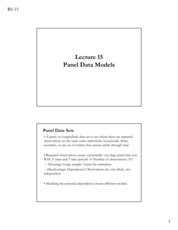
RS-15Lecture 15Panel Data ModelsPanel Data Sets A panel, or longitudinal, data set is one where there are repeatedobservations on the same units: individuals, households, firms,countries, or any set of entities that remain stable through time. Repeated observations create a potentially very large panel data sets.With N units and T time periods Number of observations: NT.– Advantage: Large sample! Great for estimation.– Disadvantage: Dependence! Observations are, very likely, notindependent. Modeling the potential dependence creates different models.1

RS-15Panel Data Sets The National Longitudinal Survey (NLS) of Youth is an example.The same respondents were interviewed every year from 1979 to 1994.Since 1994 they have been interviewed every two years. Panel data allows us a researcher to study cross section effects –i.e.,along N, variation across the firms- & time series effects –i.e., along T,variation across time.Cross section y11 y12Time series y1t y1Ty 21y 22 y 2t y 2T yi1yi 2 yit yiT y N1 y N 2 y Nt y NT Panel Data Sets Notation: x11 yi1 y11 x y y 12 12 i2 y1 ;.;yi X1 x1t yit y1t y1T yiT x1T1 w11 w21x21 . xk1 w x22 . xk2 12 w22 . ;.;Xi x2t . xk2 w1t w2t x2T1 . xkT1 w1Tj w2Tj. wk1 . xk2 . . wk2 . wkTj A standard panel data set model stacks the yi’s and the xi’s:y X c X is a ΣiTixk matrix is a kx1 matrixc is ΣiTix1 matrix, associated with unobservable variables.y and are ΣiTix1 matrices2

RS-15Panel Data Sets Financial data sets– COMPUSTAT provides financial data by firm (N 99,000) andby quarter (T 1962:I, 1962:II, ., )– CRSP daily and monthly stock and index returns from 1962 on.– Datastream provides economic and financial data for countries. Italso covers bonds and stock markets around the world.– Intra-daily data: Olsen (exchange rates) and TAQ (stock markettransaction prices). Essentially infinite T, large N.– OptionMetrics, also known as “Ivy DB”, is a database of historicalprices, implied volatility for listed stocks and option markets.– International Financial Statistics (IFS from the IMF) coverseconomic and financial data for almost all countries post-WWII.Balanced and Unbalanced Panels Notation:yi,t, i 1, ,N; t 1, ,Ti Mathematical and notational convenience:- Balanced:NT(that is, every unit is surveyed in every time period.)N- Unbalanced: i 1 TiQ: Is the fixed Ti assumption ever necessary? SUR models. The NLS of Youth is unbalanced because some individuals have notbeen interviewed in some years. Some could not be located, somerefused, and a few have died. CRSP is also unbalanced, some firms arelisted from 1962, others started to be listed later.3

RS-15Panel Data Models With panel data we can study different issues:- Cross sectional variation (unobservable in time series data) vs.Time series variation (unobservable in cross sectional data)- Heterogeneity (observable and unobservable individualheterogeneity)- Hierarchical structures (say, zip code, city and state effects)- Dynamics in economic behavior- Individual/Group effects (individual effects)- Time effectsPanel Data Models: Example 1 - SUR In Zellner’s SUR formulation (no linear dependence on yit) we have:(A1) yit xit’ i it(A2) E[ i X] 0,(A3’) Var[ i X] i2IT--groupwise heteroscedasticity.E[ it jt X] ij--contemporaneous correlationE[ it jt’ X] 0when t t’(A4) Rank(X) full rank In (A1)- (A4), we have the a GR model with heteroscedasticity. OLSin each equation is OK, but not efficient. GLS is efficient. We are not taking advantage of pooling –i.e., using NT observations! Use LR or F tests to check if pooling (aggregation) can be done.4

RS-15Panel Data Models: Example 2 - Pooling Assumptions(A1) yit xit’ zi’ γ iti 1, 2, ., Nt 1, 2, ., Ti(A2) E[ i X,z] 0,(A3) Var[ i X,z] 2I.(A4) Rank(X) full rank- the DGP- we think of i as individuals or groups.- usually, N T.- X and z: exogenous- Heteroscedasticity can be allowed. We think of X as a vector of observed characteristics. For example,firm size, Market-to-book, Z-score, R&D expenditures, etc. We think of z as a vector of unobserved characteristics (individualeffects). For example, quality of management, growth opportunities, etc.Panel Data Models: Basic Model The DGP (A1) is linear:ky it 1 j Xj 2sjit p Z pi t itp 1– Indices:- i: individuals –i.e., the unit of observation–,- t: time period,- j: observed explanatory variables,- p: unobserved explanatory variables.– Time trend t allows for a shift of the intercept over time, capturingtime effects –technological change, regulations, etc. But, if the implicitassumption of a constant rate of change is strong ( δ), we use a set ofdummy variables, one for each time period except reference period.255

RS-15Panel Data Models: Basic Model– X: The variables of interest –β is the vector of parameter of interest.– Z: The variables responsible for unobserved heterogeneity (&dependence on the yi’s). Usually, a nuisance component of the model. The Zp variables are unobserved: Impossible to obtain informationabout the pZp component of the model. We define a term c theunobserved effect, representing the joint impact of the Zp variables on yi –like an index of unobservables for individual i:s ci pZpip 1 We can rewrite the regression model as:ky it 1 jXjit c i t itj 231Panel Data Models: Basic Modelky it 1 jXjit c i t itj 2Note: If the Xj’s are so comprehensive that they capture all relevantcharacteristics of individual i, c can be dropped and, then, pooled OLSmay be used. But, this is situation is very unlikely. In general, dropping c leads to missing variables problem: bias! We usually think of c as contemporaneously exogenous to the conditionalerror. That is, E[ it c ] 0, t 1,., T A stronger assumption: Strict exogeneity can also be imposed. Then,t 1,., TE[ it xi1, xi2,.,xiT, c ] 0,306

RS-15Panel Data Models: Basic Model Strict exogeneity conditions on the whole history of xi. Under thisassumption:kE [ y it x it , c i ] 1 jXjit ci tj 2 The βj’s are partial effects holding c constant. Violations of strict exogeneity are not rare. For example, if xitcontains lagged dependent variables or if changes in it affect xit 1 (a“feedback” effect). But to estimate β we still need to say something about the relationbetween xit and c . Different assumptions will give rise to differentmodels.30Panel Data Models: Types The basic DGP:yit xit’ zi’ γ it& (A2)-(A4) apply.Depending on how we model the heterogeneity in the panel, we havedifferent models. Four Popular Models:(1) Pooled (Constant Effect) Modelzi’γ is a constant. zi α (and uncorrelated with xit!). Dependence on theyit may enter through the variance. That is, repeated observations onindividual i are linearly independent. In this case,yit xit’ α it OLS estimates α and consistently. We estimate k 1 parameters.317

RS-15Panel Data Models: Types(2) Fixed Effects Model (FEM)The zi’s are correlated with Xi Fixed Effects:E[zi Xi] g(Xi) α*i;the unobservable effects are correlated with included variables –i.e.,pooled OLS will be inconsistent.Assume zi’ γ αi (constant; it does not vary with t). Then,yit xit’ αi it the regression line is raised/lowered by a fixed amount for eachindvidual i (the dependence created by the repeated observations!). Ineconometrics terms, this is the source of the fixed-effects. We have a lot of parameters: k N. We have N individual effects!OLS can be used to estimates α and consistently.Panel Data Models: Types(3) Random Effects Model (REM)The differences between individuals are random, drawn from a givendistribution with constant parameters. We assume the zi’s areuncorrelated with the Xi. That is,(if Xi contains a constant term, μ 0 WLOG).E[zi Xi ] μAdd and subtract E[zi’ γ] μ* from (*):yit xit’ E[zi’ γ] ( zi’ γ) - E[zi’ γ] it xit’ μ* ui itWe have a compound (“composed”) error –i.e., ui it wit. This errorwit introduces contemporaneous cross-correlations across the i group. OLS estimates μ and consistently, but GLS will be efficient.8

RS-15Panel Data Models: Types(4) Random Parameters /Coefficients ModelWe introduce heterogeneity through i . But, this may introduceadditional N parameters. A solution is to model i. For example,yit xit’( hi) αi ithi is a random vector that induces parameter variation, where hi D(0,σ2hi). That is, we introduce heteroscedasticity.Now, the coefficients are different for each individual. It is possible tocomplicate the model by making them different through time: it ( hi) θtwhere θt D(0, σ2t).Estimation: GLS, MLE.Long history: Rao (1965) and Chow (1975) worked on these models.Compact Notation Compact Notation:yi X i ci iXi is a Tixk matrix is a kx1 matrixci is a Tix1 matrixyi and i are Tix1 matricesy X c Recall we stack the yi’s and Xi’s:X is a ΣiTixk matrix is a kx1 matrixc, y and are ΣiTix1 matricesOr y X* * ,withX * [X ι] * [ c]’- ΣiTix(k 1) matrix.- (k 1)x1 matrix9

RS-15Assumptions for Asymptotics (Greene) Convergence of moments involving cross section Xi.Usually, we assume N increasing, T or Ti assumed fixed.– “Fixed-T asymptotics” (see Greene)– Time series characteristics are not relevant (may be nonstationary)– If T is also growing, need to treat as multivariate time series. Rank of matrices. X must have full column rank. Xi may not, if Ti K. Strict exogeneity and dynamics. If xit contains yi,t-1 then xit cannot bestrictly exogenous. Xit will be correlated with the unobservables inperiod t-1. Inconsistent OLS estimates! (To be revisited later.)Panel Data Models: (A3’) - No Homoscedasticity We can relax assumption (A3). The new DGP model:y X* * ,with X * [X ι] - ΣiTix(k 1) matrix. * [ c]’- (k 1)x1 matrixNow, we assume (A3’) E[ ' X] Σ σ2 IΣiTi Potentially, a lot of different elements in E[ ' X] in a panel:- Individual heteroscedasticity. Usual groupwise heteroscedasticity.- Autocorrelation (Individual/group/firm) effects. Errors have arbitrarycorrelation across time for a particular individual i:- Temporal correlation (Time) effects. Errors have arbitrary correlation acrossindividuals at a moment in time (SUR-type correlation).- Persistent common shocks: Errors have some correlation between differentfirms in different time periods (but, these shocks are assumed to die outover time, and may be ignored after L periods).10

RS-15Panel Data Models: (A3’) - Error Structures To understand the different elements in Σ, consider the followingDGP for the errors, εit’s:εit θi’ft ηit ,ft D(0, σf2)& ηit ϕ ηit-1 ςit,ςit D(0, σςi2)ft : vector of random factors common to all individuals/groups/firms.θi: vector of factor loadings, specific to individual i.ςit: random shocks to individual i, uncorrelated across both i and t.ηit: random shocks to i. This term generates autocorrelation effects in i. θi’ft generates both contemporaneous (SUR) and time-varying crosscorrelations between i and j . (Autorrelations die out after L periods.)- If ft is uncorrelated across t only contemporaneous (SUR) effects.- If ft is persistent in t both SUR and persistent common effects.Panel Data Models: (A3’) - Error Structures Different forms for E[ ' X]:- Individual heteroscedasticity.E[ i2 X] σi2 standard groupwise heteroscedasticity driven by ςit.- Autocorrelation (Individual) effects:E[ it is X] 0 (t s) auto-/time-correlation for errors, it driven by ηit.- Temporal correlation effects:E[ it jt X] 0 (i j) contemporary cross-correlation for errors driven by ft.- Persistent common shocks:E[ it js X] 0 (i j) and t s L time-varying cross-correlation for errors driven by ft. Remark: Heteroscedasticity points to GLS efficient estimation, but, asbefore, for consistent inferences we can use OLS with (adjusted forpanels) White or NW SE’s.11