Transcription
Inflation and the Price of Real Assets Matteo LeombroniMonika PiazzesiCiaran RogersMartin SchneiderJanuary 2020AbstractIn the 1970s, U.S. asset markets witnessed (i ) a 25% dip in the ratio of aggregate householdwealth relative to GDP and (ii ) negative comovement of house and stock prices that drove a 20%portfolio shift out of equity into real estate. This study uses an overlapping generations model withuninsurable nominal risk to quantify the role of structural change in these events. We attribute thedip in wealth to the entry of baby boomers into asset markets, and to the erosion of bond portfoliosby surprise inflation, both of which lowered the overall propensity to save. We also show that theGreat Inflation led to a portfolio shift by making housing more attractive than equity. Disagreementabout inflation across age groups matters for the size of tax effects, the volume of nominal credit,and the price of housing as collateral. Department of Economics, Stanford University, leombm@stanford.edu, piazzesi@stanford.edu, ciaran@stanford,schneidr@stanford. For comments and suggestions, we thank Joao Cocco, Jesus Fernandez-Villaverde, John Heaton, Susan Hume McIntosh, Larry Jones, Patrick Kehoe, Per Krusell, Ricardo Lagos, Ellen McGrattan, Toby Moskowitz, Neng Wang,and many seminar and conference participants.1
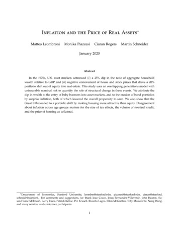
IIntroductionThe 1970s brought dramatic changes in the size and composition of US household sector wealth. Figure1 plots key household sector positions over the postwar period. During the 1970s, household net worthas a fraction of GDP fell by 25%, before recovering again to its late 1960s value. Figure 2 zooms in onthis era and shows portfolio weights in Panel (a), in particular a 20pp shift away from equity and intoreal estate during. This portfolio adjustment was largely driven by negative comovement of asset prices– house prices rose while equity prices fell, as shown in Panel (b). Compared to the big swings in themajor real asset positions, households’ net position in nominal credit instruments was relatively stable.As documented below, the stability of net positions masks substantial increases in gross borrowing andlending within the household sector.This paper studies the turbulence of the 1970s using an asset pricing model with heterogenousagents and incomplete markets. We consider overlapping generations of households who invest inequity and housing and who borrow and lend in nominal credit instruments. We fit the model to microdata on US households’ income and portfolio positions and then perform counterfactuals to understandthe 1970s. We attribute the wide swings in asset prices – and thereby household wealth – to two eventsunique to that decade: the entry of the young baby boomers into asset markets and the Great Inflationthat altered the distribution of real returns on credit for nominal borrowers and lenders. We showhow those events contribute to a lower average savings rate as well as a portfolio shift towards housingfor the aggregate household sector. At the same time, the outstanding quantity of houses, equity andgovernment debt declined only slightly; shifts in household asset demand thus resulted in large priceadjustments.Individual asset demand in our model comes from a life cycle consumption savings problem withuninsurable income risk and portfolio choice between housing, equity and nominal bonds. Householdscan borrow only against housing, not against equity or human wealth (that is, permanent income).This feature helps to match that (i) many households have a lot debt, but positive net worth and (ii)younger and poorer households who have low financial wealth relative to permanent income saveless out of financial wealth. We further work with a standard income process: most income riskis idiosyncratic so human wealth is not very exposed to aggregate shocks moving house and stockprices. This feature helps match observed portfolio choice: younger households build riskier financialportfolios, in particular through leveraged investment in housing. This is optimal because they haverelatively more human wealth that is not exposed to asset price movements.Our asset pricing results reflect how demographics and the Great Inflation altered both savings andportfolio choice. First, savings declined because there were relatively more young households, andbecause surprise inflation eroded the financial wealth of nominal lenders. Second, beliefs about futureinflation induced a portfolio shift towards housing. A prominent reason is that nominal rigidities inthe tax code favor housing over equity in times of high expected inflation. Moreover, survey data showthat households disagreed about expected inflation: young borrowers expected higher inflation – andhence lower real interest rates – than old lenders. The resulting gains from trade in the nominal credit2
3.53Net Worth/GDP2.521.5Housing/GDP1Equity/GDP0.5Net Nominal Assets/GDP196019701980199020002010Figure 1: Aggregate wealth components (market value) divided by GDP, Financial Accounts of theUnited States & own computations, 1952:1-2016:4.market increased credit and pushed up the price of collateral. At the same time, inflation uncertaintyprovided an important counterforce that dampened the response of credit.Our empirical strategy uses micro data on household characteristics to directly parameterize household sector asset demand. Our model describes three 6-year trading periods, highlighted in yellow inFigures 1-2. For each trading period, we estimate the distribution of income and initial asset endowments across households from the Survey of Consumer Finances (SCF). We parameterize beliefs aboutfuture prices and income using a mix of historical data and survey forecasts. We can then compute optimal household asset demand functions given prices, endowments and expectations. Finally, we findequilibrium prices for the trading period to equate aggregate household asset demand to the (observed)quantity of assets supplied to households by other sectors, measured using the Financial Accounts ofthe United States (FAUS).To establish that the model is a useful tool for thinking about asset pricing with heterogeneousagents, we check its ability to match not only prices but a rich cross section of household savings andportfolio choices. We select preference parameters so the model closely replicates the aggregate wealthto-GDP ratio, household sector portfolio weights, as well as the nominal interest rate in 1995. It thenalso matches price dividend ratios for both equity and real estate. The success of the model is that it3
0.7Housing0.60.50.4Equity0.30.2Net nominal assets0.11955 1960 1965 1970 1975 1980 1985 1990 1995 2000(a) Aggregate Portfolio Shares4540Equity35302520Housing15101955 1960 1965 1970 1975 1980 1985 1990 1995 2000(b) Price-dividend ratio and price-rent ratioFigure 2: Financial Accounts of the United States & own computations, 1952:1-2003:44
captures a number of (untargeted) stylized facts about the cross-section of households in the 1995 SCF.In particular, it generates hump-shaped cohort market shares in wealth, real estate and equity, as wellas net nominal positions that increase – and real estate shares that decrease – with age and net worth.The main mechanism behind these facts is that agents who expect more future non-asset income arewilling to build more risky portfolios.Counterfactuals that vary endowments, supply or expectations then serve to show the quantitativeimportance of each element for price fluctuations. In particular, we use the model to examine the1970s. We first show that it produces a drop in aggregate wealth between 1968 and 1978 for a widerange of expectation scenarios. It attributes the dip in the wealth-GDP ratio to two effects. First, theentry of baby boomers into asset markets lowered the average savings rate. Second, capital losses fromrealized inflation lowered wealth and hence savings, especially for older households. At the same time,lower savings were not counteracted by a large increase in interest rates, because the outside supply ofbonds to the household sector also fell – the main force here is a reduction of government debt. Here,measurement of asset supply is crucial for the quantitative results.Our quantitative analysis implies that both inflation expectations and inflation uncertainty wererelevant for asset prices and household positions in the 1970s, while neither can account for the databy itself. When we simply endow agents with cohort median inflation expectations from the MichiganSurvey, our model predicts a portfolio shift towards housing very close to what we see in the data.However, it also generates counterfactually high credit volumes and nominal interest rate. Inflationuncertainty is a plausible feature of beliefs that makes trading in nominal credit less attractive. Ourpreferred specification for beliefs combines the two forces to account jointly for household wealth,portfolio weights, credit volumes and prices.Our methodological approach differs from other studies of asset pricing with heterogeneous agentsand may be interesting in its own right. Our goal is to characterize asset prices that are consistent withhousehold optimization. We share this goal with conventional analysis of Euler equations pioneered byHansen and Singleton (1982) that relates asset prices to the dynamics of consumption. The differenceis that we relate asset prices to the distribution of household characteristics and the supply from othersectors, trading period by trading period. However, like Hansen and Singleton, we examine a set ofrelationships between observables that must hold in general equilibrium as long as households solveour life cycle problem. Our theory thus has content even if we do not take a stand on the behavior ofother sectors, such as the government, businesses and the rest of the world, much like Euler equationtests have content even if the dynamics of consumption are taken from the data.A novel feature of our approach is that the distribution of the key endogenous state variable thatdrives individual savings and portfolio choice – financial wealth relative to permanent income – comesdirectly from the data. We can thus provide a new perspective on the role of heterogeneity for assetprices. Existing studies have shown that heterogeneity does not matter if asset demand functionsare approximately linear over the support of a model-implied wealth distribution. We examine assetdemand in the support of the observed wealth distribution. We find that while approximate aggregation5
obtains within all but the youngest age cohorts, the distribution of wealth across cohorts matters a lot,as emphasized by Krueger and Kubler (2004).The idea that demographics should matter for asset prices in theory has been discussed for a longtime, although there is no consensus on its quantitative impact. Several studies have shown that demographics cannot fully account for changes in stock prices if equity is the only long-lived asset in themodel (Abel, 2003, Geanakoplos, Magill and Quinzii, 2004). The effect of demographics on house priceshas been explored by Mankiw and Weil (1989) as well as Ortalo-Magne and Rady (2006). A recent literature on the Great Stagnation argues that low real interest rates reflect the aging of baby boomers(for example, Gagnon, Johannsen and Lopez-Salido, 2016, or Eggertsson, Mehrotra and Robbins, 2019).These studies model the savings margin and the relationship between growth and real interest rates.Our focus is on portfolio choice and asset price fluctuations in a world with multiple long-lived assetsthat incur capital gains and losses.1 With both equity and real estate present in nonzero net supply,demographic shifts impact aggregate savings and hence the wealth-GDP ratio, but they cannot accountfor the larger movements in the individual components of wealth, especially equity.The effects of inflation on (real) asset prices is also a familiar theme in the literature. We buildon earlier work that has stressed the interaction of taxes and inflation, in particular, Feldstein (1980),Summers (1981) and Poterba (1991). We evaluate the role of nominal rigidities in the tax code ina life cycle setup when agents disagree about inflation. Our assumptions on disagreement by ageare consistent with Malmendier and Nagel (2016) who attribute it to households’ updating beliefs overtheir lifetime. We show that disagreement interacts importantly with taxes: the fact that old householdswho hold most equity expected lower inflation reduces the strength of tax-driven portfolio shifts. Wefurther emphasize that disagreement and inflation uncertainty have opposite effects on nominal creditvolumes. The role of inflation uncertainty in the 1970s has been emphasized by Cogley and Sargent(2001).There is a large body of work on quantitative asset pricing models with heterogeneous agents andincomplete markets. Its main focus is the properties of equity and bond returns in stationary rational expectations equilibria with real shocks, following the classic contributions of Constantinides andDuffie (1996), Heaton and Lucas (1996), and Krusell and Smith (1998). Constantinides et al. (2002), andStoresletten, Telmer and Yaron (2007) consider OLG models with equity, riskless bonds and uninsurableincome risk. Favilukis, Ludvigson and van Nieuwerburgh (2017) also allow for housing in a productioneconomy. Chien, Cole and Lustig (2012, 2016) study models with different perceptions and constraints,and hence disagreement about asset payoffs. We share with this literature the theme that movementsof the wealth distribution can matter for prices, as the identity of the average investor changes. Ourapproach of measuring that distribution directly clarifies the strength of this mechanism. We furtherdiffer from this literature in our focus on the 1970s and the unique events that shaped it.A recent literature studies the boom-bust episodes of the
Inflation and the Price of Real Assets Matteo Leombroni Monika Piazzesi Ciaran Rogers Martin Schneider January 2020 Abstract In the 1970s, U.S. asset markets witnessed (i) a 25% dip in the ratio of aggregate household wealth relative to GDP and (ii) negative comovement of house and stock prices that drove a 20% portfolio shift out of equity into real estate. This study uses an overlapping .