WIXLIB

Journal of Glaciology, Vol. 54, No. 184, 200817An investigation into the forces that drive ice-shelf rift propagationon the Amery Ice Shelf, East AntarcticaJeremy N. BASSIS,1 Helen A. FRICKER,1 Richard COLEMAN,2,3,4Jean-Bernard MINSTER11Institute for Geophysics and Planetary Physics, Scripps Institution of Oceanography,University of California–San Diego, La Jolla, California 92093-0225, USAE-mail: jbassis@ucsd.edu2Center for Marine Science, University of Tasmania, Hobart, Tasmania 7000, Australia3CSIRO Marine and Atmospheric Research, Box 1538, Hobart, Tasmania 7001, Australia4Antarctic Climate and Ecosystems CRC, Box 252-80, Hobart, Tasmania 7001, AustraliaABSTRACT. For three field seasons (2002/03, 2004/05, 2005/06) we have deployed a network of GPSreceivers and seismometers around the tip of a propagating rift on the Amery Ice Shelf, East Antarctica.During these campaigns we detected seven bursts of episodic rift propagation. To determine whetherthese rift propagation events were triggered by short-term environmental forcings, we analyzedsimultaneous ancillary data such as wind speeds, tidal amplitudes and sea-ice fraction (a proxy variablefor ocean swell). We find that none of these environmental forcings, separately or together, correlatedwith rift propagation. This apparent insensitivity of ice-shelf rift propagation to short-term environmental forcings leads us to suggest that the rifting process is primarily driven by the internalglaciological stress. Our hypothesis is supported by order-of-magnitude calculations that theglaciological stress is the dominant term in the force balance. However, our calculations also indicatethat as the ice shelf thins or the rift system matures and iceberg detachment becomes imminent, shortterm stresses due to winds and ocean swell may become more important.1. INTRODUCTIONThe fourth Intergovernmental Panel on Climate Change(IPCC) assessment report concluded that the Antarctic icesheet is losing mass, but that current estimates of mass lossare highly uncertain (Lemke and others, 2007). The reportemphasized deficiencies in our understanding of relativelyrapid (i.e. decades to century scale) changes occurring atice-sheet margins and did not include these dynamic icesheet changes in its sea-level projections. This has exposedan urgent need to improve our understanding of processesacting at the margins of the ice sheets.In Antarctica, the primary mechanism for mass loss isiceberg calving ( 75%); the other major mass-loss mechanism is basal melting ( 25%) (Jacobs and others, 1992).Basal melt rates have been estimated for most of the majorice shelves (e.g. Joughin and Padman, 2003), but calvingrates are more uncertain. The timescale between majoriceberg calving events on ice shelves is long (typicallyseveral decades), and such events form part of the naturalcycle of advance (by ice flow) and retreat (by calving) of theice front. Although major calving events occur sporadically,when they do occur they remove large amounts of mass in anear-instantaneous fashion. Thus a small increase in thefrequency of large calving events could lead to substantialnegative mass balance. Furthermore, the acceleration oftributary glaciers in the wake of the collapse of the Larsen Bice shelf in the Antarctic Peninsula (Rignot and others, 2004;Scambos and others, 2004) has demonstrated that ice shelvesare not merely passive indicators of climate change, but aredynamically coupled to flow of inland ice and capable ofmodulating ice flow far upstream of the grounding line. Thus,even though the retreat or loss of ice shelves does notsignificantly affect sea-level rise, their demise affects thedischarge of grounded ice, which contributes directly to sealevel rise.It is known that the calving process involves the initiationand propagation of large-scale ‘rifts’, i.e. fractures thatpenetrate the entire ice thickness, and that ice-shelf rifts canpropagate horizontally for decades before multiple riftsisolate an iceberg. However, very little is known about theforces and mechanisms controlling rift propagation, alimitation primarily due to the paucity of available observations. The rift propagation process is clearly linked to flowdynamics over a wide range of environmental conditions,flow regimes and spatial domains. However, the details ofthis connection are not yet known, and there is debate aboutsuch basic questions as what forces drive rift propagation(Larour and others, 2004; Bassis and others, 2005; Joughinand MacAyeal, 2005; MacAyeal and others, 2007). Withoutthis knowledge, it is impossible to formulate a mathematicalmodel of iceberg calving, or to realistically incorporatethe process into larger-scale numerical ice-sheet/ice-shelf/ocean models.Since ice shelves are in contact with both the atmosphereand the ocean, there are a number of environmental forcesthat may drive rift propagation in addition to the large-scaleglaciological stress caused by the gravitational spreading ofthe ice. For instance, it has been suggested that flexuralgravity waves may trigger rift propagation (Holdsworth andGlynn, 1978; Goodman and others, 1980), a theory that wasresurrected when MacAyeal and others (2007) noticed thatthe break-up of iceberg B15A correlated with the arrival of alarge pulse of ocean swell. Vertical tidal oscillations maybend the ice, inducing stresses that, if large enough, maytrigger rift propagation. At the base of the ice shelf, tidallyDownloaded from https://www.cambridge.org/core. 28 Jun 2021 at 05:45:02, subject to the Cambridge Core terms of use.

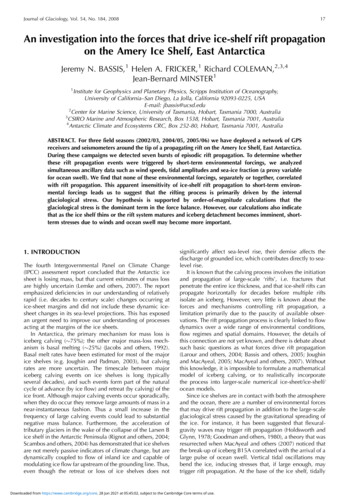
18Bassis and others: Forces that drive rift propagationFig. 2. Diagram showing the relative positions of observing stations(gray triangles) relative to the tip of rift T2 (gold star) for seasons 2and 3. Different stations and a different geometry were used for season 1. However, the network was centered on the rift tip each season.Fig. 1. (a) MODIS (moderate-resolution imaging spectroradiometer)image acquired on 18 January 2006 showing the Amery Ice Shelfand the ‘Loose Tooth’ rift system. White squares show the positionof the three ice-shelf-based AWS sites, AM01, AM02 and G3.(b) Line map showing the location of the Amery Ice Shelf in EastAntarctica. The tide gauge was located at Davis. (c) Landsat imageacquired on 18 December 2002 showing a close-up of theLoose Tooth rift system. The L1–T1–T2 triple junction was firstobserved in 1995. Since then L1 has widened but has not increasedin length.driven sub-ice-shelf currents exert a drag force which couldinduce propagation. At the ice-shelf surface, the cold denseair from katabatic winds (blowing down onto the ice shelfand across the rift) combined with large Antarctic stormsystems can produce large wind fields that also result insubstantial frictional drag force. When either of these twodrag forces (basal or surface) is integrated over a largeenough area, it may result in a substantial stress applied tothe ice shelf. In addition to the above variables that directlyexert a stress on the ice shelf, there are variables thatindirectly modulate the stress. The presence of sea ice, forexample, will dampen the amplitude of ocean swell(Wadhams, 2000), and above-freezing atmospheric temperatures may promote hydro-fracturing of the ice via theproduction of surface melt (Scambos and others, 2003; Alleyand others, 2005).Thus the crucial first step in improving our knowledge oficeberg calving is identifying which force(s) are responsiblefor driving rift propagation. To achieve this, we deployed adensely spaced network of seismometers and global positioning system (GPS) receivers around the tip of a propagating rift on the Amery Ice Shelf, East Antarctica, for threeaustral summer field seasons (Bassis and others, 2005,2007). Our observing network was supplemented by automatic weather stations (AWS) and tide gauges operated bythe Australian Antarctic Division (AAD). This instrumentation provided us with ancillary observations of relevantenvironmental variables, against which we could compareour network data. We augment the field component of thisstudy with a time series of satellite-derived rift lengthspublished by Fricker and others (2005) and extendedthrough 2006. These data provide additional informationabout the rift propagation rate on longer timescales (monthlyand longer).2. AMERY ICE SHELF RIFT-MONITORINGPROGRAM (2003–07)2.1. Location of study and instrumentationOur field study was designed to monitor a system of rifts thathave formed near the front of the Amery Ice Shelf (Fig. 1).The rift system consists of two longitudinal-to-flow rifts 30 km apart that initiated about 20 years ago (L1 and L2)and two transverse-to-flow rifts (T1 to the west and T2 to theeast) that initiated at the tip of L1, forming a triple junctionfirst observed in 1996 (Fricker and others, 2002). This riftsystem forms the outline of an intermediate-sized iceberg(30 km by 30 km), termed the ‘Loose Tooth’, that is expectedto detach within the next decade. Rift T2 currently propagates at approximately 4 m d–1, and when T2 connects withL2, the Loose Tooth iceberg will likely detach.Our field site was located near the tip of T2, where wedeployed a network of seismometers and GPS receiversduring each austral summer season. The geometry of onesuch deployment is shown in Figure 2. Although our instrumentation and network geometry varied each season, thecenter of the network was translated to correspond to theapproximate location of the rift tip observed in the field. In2002/03 we deployed eight stations which acquired data for42 days: six with a single-component L-4C seismometerrecording at 10 Hz (0.1 s) and a dual-frequency GPS receiverrecording at 0.033 Hz (30 s), and two seismometer-onlystations. In 2004/05 and 2005/06 we increased the numberof stations to twelve, each with a three-component L-28seismometer, digitized with a Quanterra Q330 data loggerand a dual-frequency GPS receiver recording at 0.5 Hz (2 s)for 52 and 81 days respectively. Hereafter we refer to thethree field seasons as follows: 2002/03 is ‘season 1’; 2004/05 is ‘season 2’; 2005/06 is ‘season 3’. To facilitate comparison of timing between field seasons, we reference daysof our survey relative to day of year (DOY) 332. In additionto our observing stations, the AAD operated AWS on theAmery Ice Shelf, one located 100 km upstream from ournetwork (shown in Fig. 1).2.2. Previous resultsFieldworkWe have previously shown that over the three field seasonsof our measurements we detected seven bursts of riftpropagation: three during season 1, three during season 2Downloaded from https://www.cambridge.org/core. 28 Jun 2021 at 05:45:02, subject to the Cambridge Core terms of use.