WIXLIB

iReal-Time RenderingFourth EditionOnline appendices: Linear Algebra and Trigonometryversion 1.1; July 19, 2018Download latest from http://realtimerendering.comTomas Akenine-MöllerEric HainesNaty HoffmanAngelo PesceMichal IwanickiSébastien Hillaire

ContentsA SomeA.1A.2A.3A.4A.5Linear AlgebraEuclidean Space . . . . . .Geometrical InterpretationMatrices . . . . . . . . . .Homogeneous Notation . .Geometry . . . . . . . . .11381516B TrigonometryB.1Definitions . . . . . . . . . . . . . . . . . . . . . . . . . . . . . . . .B.2Trigonometric Laws and Formulae . . . . . . . . . . . . . . . . . .232325References29Bibliography31Index32.iii.

Appendix ASome Linear AlgebraBOOK I. DEFINITIONS.A point is that which has no part.A line is a breadthless length.The extremities of a line are points.A straight line is a line which lies evenly with the points on itself.—The first four definitions from Elements by Euclid [4]This appendix deals with the fundamental concepts of linear algebra that are of greatest use for computer graphics. Our presentation will not be as mathematically abstractand general as these kinds of descriptions often are, but will rather concentrate on whatis most relevant. For the inexperienced reader, it can be seen as a short introductionto the topic, and may otherwise serve as a review.We will start with an introduction to the Euclidean spaces. This may feel abstractat first, but in the section that follows, these concepts are connected to geometry,bases, and matrices. So, bite the bullet during the first section, and reap the rewardsin the rest of the appendix and in many of the other chapters of this book.A.1 Euclidean SpaceThe n-dimensional real Euclidean space is denoted Rn . A vector v in this space is ann-tuple, that is, an ordered list of real numbers: v0 v1 v Rn v . with vi R, i 0, . . . , n 1.(A.1) . vn 1Note that the subscripts start at 0 and end at n 1, a numbering system thatfollows the indexing of arrays in many programming languages, such as C and C .1

2A. Some Linear AlgebraThis makes it easier to convert from formula to code. Some computer graphics booksand linear algebra books start at 1 and end at n.The vector can also be presented as a row vector, but most computer graphics textsuse column vectors, in what is called the column-major form. We call v0 , . . . , vn 1the elements, the coefficients, or the components of the vector v. All bold lowercaseletters are vectors that belong to Rn , and italicized lowercase letters are scalars thatbelong to R. As an example, a two-dimensional vector is v (v0 , v1 )T R2 . Forvectors in a Euclidean space there exist two operators, addition and multiplication bya scalar, which work as might be expected: u0v0u0 v0 u1 v1 u1 v1 (A.2)u v . . Rn (addition). . . .un 1vn 1un 1 vn 1and au au0au1. Rn (multiplication by a scalar).(A.3)aun 1nThe “ R ” simply means that addition and multiplication by a scalar yields vectorsof the same space. As can be seen, addition is done componentwise, and multiplicationis done by multiplying all elements in the vector with the scalar a.A series of rules hold for Euclidean space—in fact, these are the definition ofEuclidean space. Addition of vectors in a Euclidean space also works as might beexpected:(i) (u v) w u (v w) (associativity)(A.4)(ii) u v v u(commutativity).There is a unique vector, called the zero vector, which is 0 (0, 0, . . . , 0) with nzeros, such that(iii) 0 v v (zero identity).(A.5)There is also a unique vector v ( v0 , v1 , . . . , vn 1 ) such that(iv) v ( v) 0(additive inverse).(A.6)Rules for multiplication by a scalar work as follows:(i) (ab)u a(bu)(ii) (a b)u au bu(iii) a(u v) au av(iv) 1u ultiplicative one).(A.7)

A.2. Geometrical Interpretation3For a Euclidean space we may also compute the dot product of two vectors u andv. This value is also called inner (dot) product or scalar product. The dot product isdenoted u · v, and its definition is shown below:u · v u v cos φ(dot product),(A.8)where u · v 0 if u 0 or v 0. Here, φ (shown at the left in Figure A.3)is the smallest angle between u and v. Several conclusions can be drawn from thesign of the dot product, assuming that both vectors have non-zero length. First,u · v 0 u v, i.e., u and v are orthogonal (perpendicular) if their dot productis zero. Second, if u · v 0, then it can seen that 0 φ π2 , and likewise if u · v 0then π2 φ π. For the dot product we have the rules:(i)(ii)(iii)(iv)(v)u · u 0, with u · u 0 if and only if u (0, 0, . . . , 0) 0(u v) · w u · w v · w(distributivity)(au) · v a(u · v)(associativity)u·v v·u(commutativity)u · v 0 u v.(A.9)The last formula means that if the dot product is zero then the vectors are orthogonal(perpendicular).A.2 Geometrical InterpretationHere, we will interpret the vectors (from the previous section) geometrically. For this,we first need to introduce the concepts of linear independence and the basis. If theonly scalars to satisfy Equation A.10 below are v0 v1 . . . vn 1 0, then thevectors, u0 , . . . un 1 , are said to be linearly independent. Otherwise, the vectors arelinearly dependent:v0 u0 · · · vn 1 un 1 0(A.10)For example, the vectors u0 (4, 3) and u1 (8, 6) are not linearly independent,since v0 2 and v1 1 (among others) satisfy Equation A.10. Only vectors thatare parallel are linearly dependent.If a set of n vectors, u0 , . . . , un 1 Rn , is linearly independent and any vectorv Rn can be written asn 1Xv vi ui ,(A.11)i 0then the vectors u0 , . . . , un 1 are said to span Euclidean space Rn . If, in addition,v0 , . . . , vn 1 are uniquely determined by v for all v Rn , then u0 , . . . , un 1 is calleda basis of Rn . What this means is that every vector can be described uniquely byn scalars (v0 , v1 , . . . , vn 1 ) and the basis vectors u0 , . . . , un 1 . The dimension of thespace is n, if n is the largest number of linearly independent vectors in the space.

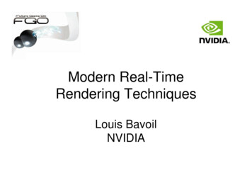
4A. Some Linear AlgebraFigure A.1. A three-dimensional vector v (v0 , v1 , v2 ) expressed in the basis formed by u0 , u1 , u2in R3 . Note that this is a right-handed system.An example of a linearly independent basis is u0 (4, 3) and u1 (2, 6). Thisspans R2 , as any vector can be expressed as a unique combination of these two vectors. For example, ( 5, 6) is described by v0 1 and v1 0.5 and no othercombinations of v0 and v1 .To completely describe a vector, v, one should use Equation A.11, that is, using both the vector components, vi and the basis vectors, ui . That often becomesimpractical, and therefore the basis vectors are often omitted in mathematical manipulation when the same basis is used for all vectors. If that is the case, then v can bedescribed as v0 v1 v . ,(A.12) . vn 1which is exactly the same vector description as in Expression A.1, and so this isthe one-to-one mapping of the vectors in Section A.1 onto geometrical vectors. Anillustration of a three-dimensional vector is shown in Figure A.1. In this book, a vectorv can thought of as a point in space or as a directed line segment (i.e., a directionvector). All rules from Section A.1 apply in the geometrical sense, too. For example,the addition and the scaling operators from Equation A.2 are visualized in Figure A.2.A basis can also have different “handedness.”A three-dimensional, right-handed basis is one in which the x-axis is along thethumb, the y-axis is along index-finger, and the z-axis is along the middle finger. Ifthis is done with the left hand, a left-handed basis is obtained. See page 11 for a moreformal definition of “handedness.”Now we will go back to the study of basis for a while, and introduce a special kindof basis that is said to be orthonormal. For such a basis, consisting of the basis vectorsu0 , . . . , un 1 , the following must hold: 0, i 6 j,ui · uj (A.13)1, i j.

A.2. Geometrical Interpretation5Figure A.2. Vector-vector addition is shown in the two figures on the left. They are called the headto-tail axiom and the parallelogram rule. The two rightmost figures show scalar-vector multiplicationfor a positive and a negative scalar, a and a, respectively.This means that every basis vector must have a length of one, i.e., ui 1, and thateach pair of basis vectors must be orthogonal, i.e., the angle between them must be π/2radians (90 ). In this book, we mostly use two- and three-dimensional orthonormalbases. If the basis vectors are mutually perpendicular, but not of unit length, then thebasis is called orthogonal. Orthonormal bases do not have to consist of simple vectors.For example, in precomputed radiance transfer techniques the bases often are eitherspherical harmonics or wavelets. In general, the vectors are exchanged for functions,and the dot product is augmented to work on these functions. Once that is done, theconcept of orthonormality applies as above.For an orthonormal basis, the dot product (Equation A.8) can be simplified to:u·v n 1Xui vi(dot product).(A.14)i 0Let p (p0 , . . . , pn 1 ), then for an orthonormal basis it can also be shown thatpi p · ui . This means that if you have a vector p and a basis (with the basis vectorsu0 , . . . , un 1 ), then you can easily get the elements of that vector in that basis bytaking the dot product between the vector and each of the basis vectors. The mostcommon basis is called the standard basis, where the basis vectors are denoted ei .The ith basis vector has zeros everywhere except in position i, which holds a one. Forthree dimensions, this means e0 (1, 0, 0), e1 (0, 1, 0), and e2 (0, 0, 1). We alsodenote these vectors ex , ey , and ez , since they are what we normally call the x-, they-, and the z-axes.The norm of a vector, denoted u , is a non-negative number that can be expressedusing the dot product:r Pn 1 2 (A.15) u u · u (norm).i 0 ui

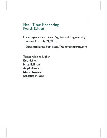
6A. Some Linear AlgebraFigure A.3. The left figure shows the notation and geometric situation for the dot product. In therightmost figure, orthographic projection is shown. The vector u is orthogonally (perpendicularly)projected onto v to yield w.However, this is only true for an orthonormal basis. For the norm, we have:(i)(ii)(iii)(iv) u 0 u (0, 0, . . . , 0) 0 au a u u v u v (triangle inequality) u · v u v (Cauchy–Schwartz inequality).(A.16)The norm of a vector (see Equation A.15) can be thought of as the lengthp of thevector. For example, the length of a two-dimensional vector, u, is u u20 u21 ,is computed using the Pythagorean theorem. To create a vector of unit length, i.e.,of length one, the vector has to be normalized. This can be done by dividing by the1p, where q is the normalized vector, which also is calledlength of the vector: q p a unit vector.A useful property of the dot product is that it can be used to project a vectororthogonally onto another vector. This orthogonal projection (vector), w, of a vectoru onto a vector v is depicted on the right in Figure A.3. For arbitrary vectors u andv, w is determined by u · v u·vw v v tv,(A.17) v 2v·vwhere t is a scalar. The reader is encouraged to verify that Expression A.17 is indeedcorrect, which is done by inspection and the use of Equation A.8. The projection alsogives us an orthogonal decomposition of u, which is divided into two parts, w and(u w). It can be shown that w (u w), and of course u w (u w) holds. Anadditional observation is that if v is normalized, then the projection is w (u · v)v.This means that w u · v , i.e., the length of w is the absolute value of the dotproduct between u and v.