WIXLIB

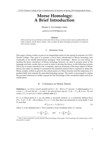
CUNY Hunter College Dpt of Mathematics & Statistics Spring 2016 Independent StudyMorse Homology:A Brief IntroductionMario L. Gutierrez Abedgutierrez.m101587@gmail.comAbstractAfter presenting some preliminary results from Morse theory, we discuss topics such as gradient fields, theSmale condition, and the Morse complex. Then we define the Morse homology and showcase its usefulnesswith concrete examples.I.IntroductionThis paper is being written as part of an independent study for the spring’16 semester at CUNYHunter College. Our goal is to present a (very) basic introduction to Morse homology and,eventually, to its infinite-dimensional analogue: Floer homology.1 Before we even dream oftackling the heavy machinery of Morse homology however, we need to present some of thelanguage and basic results that we need in order to develop the theory in the following sections.This is by no means intended to be a complete, rigorous treatment of the deep subject of Morsetheory, but rather an attempt to summarize the essential material that is required to define theMorse complex (which is given by the critical points of a Morse function and the trajectories of agradient field) and compute the associated homology groups. The reader is encouraged to explorethe provided references to further expand his/her knowledge of this wonderful subject and all itsramifications.II.A Sprinkle of Morse TheoryDefinition 1. Let M be a smooth manifold and let f : M R be a C function. A critical point of f isa point x M such that d f x 0; that is, the induced linear map d f : Tx M T f ( x) R is zero. The realnumber f ( x ) in such case is called a critical value of f .If x is a critical point of f , we can define a covariant 2-tensor, i.e. a symmetric bilinear formd2 f x : Tx M Tx M R as follows: If v, w Tx M, then there are extensions to vector fields V andW such thatd2 f x (v, w) Vx (W f ( x )),(1)where Vx is by definition just v. Now consider a local coordinate chart ( xi ) and letv V i xiixandw W j x jjx.1 Dueto time constraints we only discuss Morse homology in this paper. Floer homology and related topics will bediscussed in a sequel.1

CUNY Hunter College Dpt of Mathematics & Statistics Spring 2016 Independent Study(We can also take W j W j / x j , where W j is now a constant function.) Then,2d f x (v, w) Vx (W f ( x )) v(W f )( x ) vso that the matrix f W x jj!j 2 f(x) xi x j(x) V i W ji,j 2 f( x ), xi x j (2)represents d2 f x with respect to the basis / x1 x , . . . , / x n x . (This matrix is known as theHessian of f .)Definition 2. We will say that a critical point x is degenerate if the bilinear form d2 f x is degenerate(i.e. if d2 f x 0); we call x nondegenerate otherwise. Moreover, we will say that a function is a Morsefunction if all its critical points are nondegenerate.Remark 1. It is clear that a critical point x is nondegenrate if and only if the matrix (2) is nonsingular(i.e. invertible).It is a fact that studying a well-chosen function on a manifold can give rather precise informationon its topology. A most instructive example is known as the "height" function f : R3 R and itsrestriction f to the different submanifolds embedded (or immersed) in R3 , as presented in thefollowing figures. 1f 1In the figure above, note that for a R, the level sets of f aref 1 ( a ) if a 1, a point if a 1,a circle if 1 a 1, a point if a 1, if a 1.Each of these level sets has a well defined topology which changes exactly at the regular pointsof the function; in this case at the north pole (maximum) and the south pole (minimum) of the2-sphere. The situation is analogous for the torus T2 in the next figure, except that there are now2

CUNY Hunter College Dpt of Mathematics & Statistics Spring 2016 Independent Studycritical points that are not extrema of the function, namely the two "saddle" points b and c:af ( a)f (b)bf cf (c)f (d)dThe corresponding level sets at these saddle points b and c are curves of the form(that is,S1 S1 ), and are therefore not submanifolds (immersed or embedded). The regular, noncritical levelsets must however all be (embedded) submanifolds because of the regular level set theorem.2Let T2a be the set of all points x T2 such that f ( x ) a. Then we have the following: D2 2 S1 I (a cylinder)Ta T2 r D̊2 T2if a f (d),if f (d) a f (c),if f (c) a f (b),if f (b) a f ( a),if a f ( a).Remark 2. In order to describe the changes in the topology of T2a as a passes through the critical values off , it is convenient to consider homotopy type rather than homeomorphism type (for a somewhat detaileddiscussion the reader is referred to [MJ]).Now let us take a second look at the "height" function on the 2-sphere, although this time weconsider a "deformed" sphere, which we denote by S2 . Obviously, S2 is still diffeomorphic to S2 ,but the function now has two local maxima and a saddle point:af ( a)f (c)cbdf f (b)f (d)2 Recall that this theorem states that every regular level set of a smooth map between smooth manifolds (or of a smoothfunction to R in our particular case) is a properly embedded submanifold whose codimension is equal to the dimension ofthe codomain.3

CUNY Hunter College Dpt of Mathematics & Statistics Spring 2016 Independent StudyNote that the parity of the number of critical points of the new function is the same as that of theoriginal one (i.e., they are equal mod 2). It turns out that if we have that the critical points of ourfunction are nondegenerate (which is indeed the case for the critical points shown in our figures),then modulo 2 the number of critical points equals the Euler characteristic of the manifold, aninvariant that does not depend on the function but only on the manifold itself. However, note thatthis invariant is not especially strong:χ(S2 ) 2,χ ( T2 ) 0mod 2χ(S2 ) χ(T2 ), but it is clear that the sphere and the torus are very different manifolds even if the two admit afunction with four nondegenerate critical points (and hence the same Euler characteristic mod2). It is the concept of Witten spaces of trajectories that will allow us to present a finer invariant(known as the Morse homology HMk (V ) of a manifold V (c.f. §IV)) in the following sections.We close out this section by presenting the Morse Lemma, which is, for our purposes, the mostimportant result of Morse theory. We refer the reader to [MJ] for a proof using Hadamard’s lemma,or to [AD] for a proof that is a direct application of the implicit function theorem.Definition 3. A symmetric bilinear form g on a vector space V is said to be negative definite providedthat for v V and v 6 0, we have g(v, v) 0. The index of g on V is the largest integer that is thedimension of a subspace W V on which g W is negative definite. We will refer to the index of thesymmetric bilinear form d2 f x which we previously defined on (1) simply as the index of f at x.The Morse Lemma will show that the behavior of a function f at p can be completely described byits index:Lemma 1 (Morse Lemma). Let p M be a nondegenerate critical point for f C ( M). Then there isa local smooth chart (U, ϕ), where U is a neighborhood of p and ϕ( p) ( x1 ( p), . . . , x n ( p)) (0, . . . , 0),and such thatf ϕ 1 ( x 1 , . . . , x n ) f ( p ) νnj 1j ν 1 ( x j )2 ( x j )2 ,where ν is the index of f at p.Definition 4. A chart in whose open set the coordinates given by the Morse lemma are defined is called aMorse chart.Remark 3. An immediate result that follows from the Morse lemma is the fact that the nondegeneratecritical points of a function are isolated. This implies, in particular, that a Morse function on a compactmanifold can only have finitely many critical points.4

CUNY Hunter College Dpt of Mathematics & Statistics Spring 2016 Independent StudyIII.Pseudo-GradientsLet ( M, g) be a Riemannian manifold and recall the notion of the gradient of a function f C ( M),denoted grad f , which is given bygrad f (d f )] f gij xi x j .i,jUnraveling the definitions, we see that for any vector field X Γ ( TM), the gradient satisfiesg(grad f , X ) (grad f )[ ( X ) d f ( X ) X f .(Here we are using the "sharp" (]) and "flat" ([) operators, which are the well known musicalisomorphisms between TM and T M.) Now we have the following definition:Definition 5. Let f : M R be a Morse function on a manifold M. A pseudo-gradient field (alsoknown as pseudo-gradient adapted to f ) is a vector field V on M such that: We have d f x (Vx ) 0, where equality holds if and only if x is a critical point. In a Morse chart in the neighborhood of a critical point, V coincides with the negative gradient for thecanonical metric on Rn .This notion allows us to make the Morse charts more precise by specifying the trajectories (alsoknown as integral curves or flow lines) of a pseudo-gradient field. For example, Figure 1 shows thedifference between a maximum and a minimum critical points in a Morse chart.Figure 1: Trajectories of a pseudo-gradient field in a Morse chart at a maximum (left) and a minimum (right).Recall that a flow domain for a manifold M is an open subset D R M with the property thatfor each p M, the set D ( p) {t R (t, p) D} is an open interval containing 0. A flow onM is then a continuous map θ : D M, where D R M is a flow domain, that satisfies thefollowing group laws: for all p M, we have θ (0, p) p, and and for all s D ( p) and t D (θ (s,p))such that s t D ( p) ,θ (t, θ (s, p)) θ (t s, p).Now we make the following important definition:5

CUNY Hunter College Dpt of Mathematics & Statistics Spring 2016 Independent StudyDefinition 6. Let p M be a critical point of f C ( M). Denote by θt the associated map θt : M Mof the flow θ : D M of a pseudo-gradient. We define the stable manifold of p to be sW ( p) x M lim θt ( x ) p ,t and its unstable manifoldW u ( p) x M lim θt ( x ) p .t Remark 4. Note that with regards to stable/unstable manifolds, it only makes sense to consider D R M,i.e. we are only going to focus on global flows.Remark 5. The stable and unstable manifolds of the critical point p are submanifolds of M that arediffeomorphic to open disks. Moreover, we havedim W u ( p) codim W s ( p) Ind( p),where Ind( p) denotes the index of the point p as a critical point of f .To illustrate the concept of stable/unstable manifolds, here is a very simple example. Consider the2-sphere S2 with the height function f described earlier. Let p be the minimum (south pole) andlet q be the maximum (north pole). Then, for any pseudo-gradient field, we haveW s ( p ) S2 r { q } ,W u ( p ) { p },and similarlyW s ( q ) { q },W u ( q ) S2 r { p } .The most important property of the trajectories of a vector field is that they all connect criticalpoints of a function: all trajectories come from a critical point and go towards another criticalpoint:Proposition 1. Suppose that M is a compact manifold. Let γ : R M be a trajectory of the pseudogradient field V. Then there exist critical points c and d of f C ( M) such thatlim γ(t) ct andlim γ(t) d.t Proof. A proof can be found on [AD, 28-29].Now we are finally arriving at the main result of this section. First let us recall that on a manifoldM two embedded submanifolds S, S0 M are said to intersect transversely if for each p S S0 ,the tangent spaces Tp S and Tp S0 together span Tp M (where we consider Tp S and Tp S0 as subspacesof Tp M). We denote the intersection of two submanifolds S, S0 that meet transversally as S t S0 .6