Transcription
A Comparative Assessment of Malware Classificationusing Binary Texture Analysis and Dynamic AnalysisLakshmanan NatarajVinod YegneswaranUniversity of California, SantaBarbara, USASRI InternationalMenlo Park, USAlakshmanan nataraj@umail.ucsb.eduPhillip Porrasvinod@csl.sri.comSRI InternationalMenlo Park, USALouisiana State UniversityBaton Rouge, USAporras@csl.sri.comzhang@csc.lsu.eduJian ZhangABSTRACTKeywordsAI techniques play an important role in automated malware classification. Several machine-learning methods have been applied toclassify or cluster malware into families, based on different features derived from dynamic review of the malware. While theseapproaches demonstrate promise, they are themselves subject to agrowing array of countermeasures that increase the cost of capturing these binary features. Further, feature extraction requires a timeinvestment per binary that does not scale well to the daily volumeof binary instances being reported by those who diligently collectmalware. Recently, a new type of feature extraction, used by a classification approach called binary-texture analysis, was introducedin [16]. We compare this approach to existing malware classification approaches previously published. We find that, while binarytexture analysis is capable of providing comparable classificationaccuracy to that of contemporary dynamic techniques, it can deliver these results 4000 times faster than dynamic techniques. Alsosurprisingly, the texture-based approach seems resilient to contemporary packing strategies, and can robustly classify a large corpusof malware with both packed and unpacked samples. We presentour experimental results from three independent malware corpora,comprised of over 100 thousand malware samples. These resultssuggest that binary-texture analysis could be a useful and efficientcomplement to dynamic analysis.Malware Images, Texture Analysis, Dynamic AnalysisCategories and Subject DescriptorsD.4.6 [Security and Protection]: Invasive Software (viruses, worms,trojan horses); I.4 [Image Processing and Computer Vision]: ApplicationsGeneral TermsComputer Security, Malware, Image ProcessingPermission to make digital or hard copies of all or part of this work forpersonal or classroom use is granted without fee provided that copies arenot made or distributed for profit or commercial advantage and that copiesbear this notice and the full citation on the first page. To copy otherwise, torepublish, to post on servers or to redistribute to lists, requires prior specificpermission and/or a fee.AISec ’11 Chicago, ILCopyright 2011 ACM 978-1-4503-1003-1/1/10 . 10.00.1.INTRODUCTIONMalware binary classification is the problem of discovering whethera newly acquired binary sample is a representative of a family ofbinaries that is known (and has ideally been previously analyzedand understood) or whether it represents a new discovery (requiring deeper inspection). Perhaps the most daunting challenge in binary classification is simply the sheer volume of binaries that mustreviewed on a daily basis. In 2010, Symantec reported its 2010corpus at over 286 million [23].In order to deal with such a huge volume, it is necessary to develop systems that are capable of automated malware analysis. AItechniques, in particular machine-learning-based techniques playan important role in such analysis. Often a set of features areextracted from malware and then unsupervised learning may beapplied to discover different malware groups/families [21] or supervised learning may be applied to label future unknown malware [21, 31]. In both cases, designing a set of features that capturethe intrinsic properties of the malware is the most critical step forAI techniques to be effective, because analysis based on featuresthat can be randomized via simple obfuscation methods will notgenerate meaningful results.There are two main types of features that are commonly used inautomated malware analysis: static features based on the malwarebinary and dynamic features based on the runtime behavior of themalware. One challenge faced by static-feature analysis techniquesis wide-spread introduction of binary obfuscation techniques thatare near-universally adopted by today’s malware publishers. Binaryobfuscation, particularly in the form of binary packing, transformsthe binary from its native representation of the original source code,into a self-compressed and uniquely structured binary file, such thatnaive bindiff-style analyses across packed instances simply do notwork. Packing further wraps the original code into a protectiveshell of logic that is designed to resist reverse engineering, makingour best efforts at unpacking and static analysis an expensive, andsometimes unreliable, investment.Dynamic features based on behavioral analysis techniques offer an alternate approach to malware classification. For example,sandnets may be used to build a classification of binaries basedon runtime system call traces [30], or one may conduct classification through host and network forensic analyses of the malware asit operates [32]. Such techniques have been studied as a possible
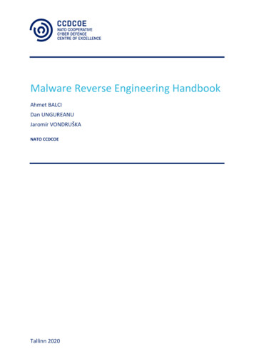
solution, but they may be challenged by a variety of countermeasures designed to produce unreliable results [22]. Dynamic analysis has also been noted to be less than robust when exposed to largedataset [14]. Consider an average dynamic analysis of a malwarebinary, in which the binary is executed, allowed to unpack, provided time to execute its program logic, and (in the worst case) issubject to full path exploration to enumerate its calling sequence,and finally terminated and its virtual machine recycled. The dynamic analysis of a single binary sample may take on the orderof 3 to 5 minutes [30] to extract the attributes used for classification. Even if such a procedure can be streamlined to 30 secondsper binary, the Symantec 2010 corpus would take over 254 years ofmachine time to process.Recently, a new type of feature has been introduced in [16] formalware classification. The approach borrows techniques from theimage processing community to cast the structure of packed binarysamples into two-dimensional grey scale images, and then uses features of this image for classification. In this paper, we compare twodifferent feature-design strategies for malware analysis, i.e., a strategy based on image-processing with dynamically derived features.What we confirm is that the binary packing systems we have analyzed perform a monotonic transformation of the binaries that failsto to conceal common structures (byte patterns) that were presentin the original binaries. We provide experiments which illustratethat the binary-texture-based strategy can produce clustering resultsroughly equivalent to the results produced by competing dynamicanalysis techniques, but at 1/4000 the amount of time per binary(from roughly 3 minutes to approximately 50ms).The image-based approach is not subject to anti-tracing, antireverse engineering logic, or many common code obfuscation strategies now incorporated into packed binaries. However, it is subjectto the coupling of the binary to the packing software. That is, astream of packed samples from a single common malware will produce a unique cluster per packer (e.g., mydoom-UPX, mydoomASPack, mydoom-PEncrypt, etc.). We believe this is quite a fairtradeoff.In section 2 we discuss the binary-texture approach to castinga binary sample into a 2D image format. In section 3 we discussdynamic analysis for generating malware classification features. Insection 4, we conduct experiments in which we compare differentstrategies for malware classification. Section 5 discusses our observations for why and how packers do not destroy the observed structures, the limitations, and possible countermeasures to the imageprocessing based technique. Section 6 presents related work, andSection 7 summarizes our results.2.BINARY TEXTURE ANALYSISAn image texture is a block of pixels which contains variationsof intensities arising from repeated patterns. Texture based features are commonly used in many applications such as medical image analysis, image classification and large-scale image search, toname a few. Recently, image texture-based classification was usedto classify malware [16]. A malware binary is first converted to animage representation on which texture based features are obtained.In this paper, we use this technique for malware classification andcompare it with current dynamic analysis based malware classification techniques. First, we briefly review the image based malwareclassification.2.1Image Representation of MalwareTo extract image-based features, a malware binary has to betransformed to an image. A given malware binary is read as a 1Darray (vector) of 8 bit unsigned integers and then organized intoa 2D array (matrix). The width of the matrix is fixed dependingon the file size and the height varies according to the file size[16].Malware Binary01110011010110010101101010100001.Binary to8 bitvector8 Bit vector toGrayscaleImageFigure 1: Block diagram to convert malware binary to an imageN 1Sub-band.Sub-bandImage.16-D Feature.16-D Feature.320-DFeatureN 20Sub-band16-D FeatureFigure 2: Block diagram to compute texture feature on an imageThe matrix is then saved as an image and the process is shown inFigure 1.2.2Texture Feature ExtractionOnce the malware binary is converted to an image, a texturebased feature is computed on the image to characterize the malware. The texture feature that we use is the GIST feature [18],which is commonly used in image recognition systems such asscene classification and object recognition [25] and large scale image search[8]. We will briefly review the computation of the GISTfeature vector. A more detailed explanation can be found in [25,18]. Figure 2 shows the block diagram to obtain the GIST feature.Every image location is represented by the output of filters tuned todifferent orientations and scales. A steerable pyramid with 4 scalesand 8 orientations is used. The local representation of an image isthen given by: V L (x) Vk (x)k 1.N where N 20 is the numberof sub-bands. In order to capture the global image properties whileretaining some local information, the mean value of the magnitudeof the local features is computed and averaged over large spatialregions: m(x) x0 V (x0 ) W (x0 x) where W (x) is the averaging window. The resulting representation is downsampled tohave a spatial resolution of M M pixels (here we use M 4). Thusthe feature vector obtained is of size M M N 320. The steps tocompute the texture feature are as follows:P1. Read every byte of a binary and store it in a numeric 1D array(range 0-255).2. Convert the 1D array to a 2D array to obtain a grayscale image. The width of the image is fixed based on the file size ofthe binary[16].3. Reshape the image to a constant sized square image of size64 64.4. Compute a 16-dimensional texture feature across for N 20sub-bands.5. Concatenate all the features to obtain a 320-dimensional feature vector.2.3Texture based Image ClassificationTexture based image features are well known in classificationof image categories. For example, in [25] GIST features are used
(a)(b)(c)(d)(e)(f)Figure 3: Sample images of 6 variants of: (a)Allaple, (b)Ejik, (c)Mydoom, (d)Tibs, (e)Udr, (f)Virutto classify outdoor scene categories. Their classification was performed using a k-nearest neighbors (k-NN) classifier, where a databaseof labeled scenes with the corresponding category called the training set is used to classify unlabeled scenes. Given a new scene,the k nearest neighbors are computed and these correspond to kscenes from the training set with the smallest distance to the testscene. Then the new scene is assigned the label of the scene category that is most represented within the k nearest neighbors. Weuse a similar approach, except that instead of outdoor scene categories, out categories correspond to malware families. The trainingset contains families of known malware. Each family further contain several malware variants. The 320-dimensional GIST featuresare computed for all the binaries in the training set. The followingalgorithm is used to classify a new unknown malware:1. The 320-dimensional GIST feature vector is computed on theunknown malware binary.2. The Euclidean Distance is computed with all feature vectorsin the training set.3. The nearest neighbors are the top k malware in the trainingset that have the smallest distance to the unknown.4. The unknown malware is assigned a label that matches a majority returned by the k labels.3.DYNAMIC FEATURE EXTRACTIONIn dynamic analysis, the behavior of the malware is traced byrunning the malware executable in a sandbox environment for several minutes. Based on the sandbox system under consideration,the type and granularity of data that is recorded might be different.In this paper, we evaluate two different dynamic analysis approaches. The first and commonly used appraoch is system-calllevel monitoring which might be implemented using API hookingor VM introspection. The system generates a sequential report ofthe monitored behavior for each binary, based on the performed operations and actions. The report typically includes all system callsand their arguments stored in a representation specifically tailoredto behavior-based analysis.Table 1: Malware datasetsDatasetHost-Rx Reference DatasetHost-Rx Application DatasetMalhuer Reference DatasetMalheur Application DatasetVXHeavens DatasetNum Binaries3932,1403,13133,69863,002Num Families624531The second approach, which we call forensic snapshot comparison relies on a combination of features that are based on comparing the pre-infection and post-infection system snapshots. Someof the key features collected include AUTORUN ENTRIES, CONNECTION PORTS, DNS RECORDS, DROP FILES, PROCESSCHANGES, MUTEXES, THREAD COUNTS, and REGISTRYMODS. A whitelisting process is used to weigh down certain commonly occurring attribute values for filenames and DNS entries. Akey difference between system-call monitoring and forensic comparison, is that the latter approach does not capture the temporalordering of forensic events. The advantage is that it is simpler toimplement and prioritize events that are deemed to be most interesting. To identify deterministic and non-deterministic features,each malware is executed three different times on different virtualmachines and a JSON object is generated describing the malwarebehavior in each execution [32]. Depending on the presence of thekey features, a binary feature vector is generated from the JSONobject. If a key feature is present in the JSON object, then corresponding component in the feature vector is 1; otherwise the component is 0. The size of the feature vector depends on the diversityof the behavior of the malware corpus, but various between 6002000 for datasets used in this paper.4.EXPERIMENTSIn this section we present several experiments that compare theresults of the binary texture analysis strategy against datasets analyzed in three separate malware binary classification efforts. Ineach experiment, every malware binary is characterized by a featurevector. We then use k-nearest neighbors (k-NN) with Euclideandistance measure for classification. The feature vectors are com-
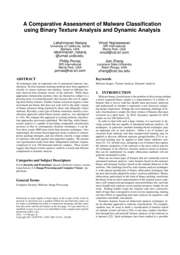
puted for all binaries in the datasets and are divided into a trainingset and a testing set. For every feature vector in the testing set, thek-nearest neighbors in the training set are obtained. Then the vectoris classified to the class which is the mode of its k-nearest neighbors. For all tests, we do a 10-fold cross validation, where undereach test, a random subset of a class is used for training and testing.For each iteration, this test randomly selects 90% data from a classfor training and 10% for testing.We summarize our datasets in Table 1. In the first experiment,Section 4.1, we compare binary texture analysis against a 2140sample dataset. Out of this 2140, we downselected 393 binariesthat have consistent labels and sufficient membership. We call thissubset the Host-Rx reference dataset which was classified using adynamic analysis technique where the binaries are clustered basedon their observed forensic impacts on the host [32]. These clustersare also examined against antivirus labels, and the minimum familysample size is 20. We employed both image analysis and dynamicanalysis on the Host-Rx dataset, recomputing the dynamic featuresand comparing the classification performance, since clustering ismainly focused in [32]. The average classification accuracy is 98%and 95% for dynamic and image analysis, respectively. Thus, wefind the binary texture technique achieves comparable success butis able to complete its feature analysis in approximately 1/4000 thetime required per binary.In the second experiment, we examine the Malhuer dataset, whichwas originally classified based on features derived by dynamic system call interception, as presented in [21]. These execution traceswere converted to a Malware Instruction Set (MIST) format, fromwhich feature vectors were extracted to effectively characterize thebinaries. Since [21] already reports the results of a malware classification based on these features, we do not repeat the dynamic analysis. In Section 4.2, we present a comparative assessment of theMalheur dataset, which includes both a reference data set of 3131malware binaries comprising 24 unique malware families, and anapplication dataset of roughly 33 thousand binaries that range frommalicious, to unknown, to known benign. Using these datasets, wefound that binary-texture classification produced comparable accuracies in both datasets, ranging from 97% for the reference set, to86% accuracy for the application set.Finally, we present a larger experiment using a VX Heavens datasetconsisting of a corpus of over 63 thousand malicious binaries comprising 531 unique families (as labeled by the Microsoft SecurityEssentials tool suite). Section 4.3 presents our results from the VXHeavens corpus, which was previously classified using the resultsfrom antivirus labels. Here the binary-texturing analysis produced a72% match with the original Microsoft AV labels. However, whilethis result may appear lower than the previous experiments, we discuss issues in the labeling and our conservative interpretation of ourbinary-texture results, which we believe account for these results.4.1Experiment 1: Binary Texture Analysis vsHost-Rx Dynamic Analysis DatasetIn this experiment, we compute the feature vectors for binarytexture analysis and forensic dump-based dynamic analysis. Weuse the Host-RX dataset [32], for this comparison.The following process was used to select malware instances withreliable labels. The initial malware corpus consisted of 2140 malware binaries. The AV labels for these binaries were obtained fromVirustotal.com [3]. Six AV vendors were used: AVG, AntiVir, BitDefender, Ikarus, Kaspersky and Microsoft. We attribute a labelto a malware instance if at least 2 AV vendors share similar labels.Out of 2140 instances, only 450 malware samples had consistentlabels. However, some malware families had very few samples.To conduct a meaningful (representative) analysis of the featurescollected, each family should have a large enough group of exem-Table 2: Family/packer summary: Host-Rx reference 0151313466Packed3111240343PackerUPX10 PeC, 1 rVirut 0.5 1 1.5 2108 2.56 32420 20 4 6 2 8 10 4Figure 5: Lower dimensional visualization of dynamic featureson Host-Rx datasetplars from which to derive consistent features. For consistency withprevious classification research ([21]) that is compared in the nextsection, we chose to remove families with less than 20 samples, andcompiled a final collection of 393 malware binaries. These binaries(shown in Table 2) represented 6 malware families. We also checkif these malware are packed or not using PeID and report the labelsin Table 2. However, some of the malware that PeID did not detectcould also be packed. Some images of the variants of the 6 familiesare shown in Figure 34.1.1Dynamic Analysis FeaturesThe dynamic analysis features are obtained from the forensicmemory dumps and then converted to a vectorial form to producea 651 dimensional vector for every malware instance, as shown inFigure 4. The result is a binary matrix, where 1 refers to the presence of a corresponding feature. The first 81 samples belong to Allaple and most of their features are between 75 and 219 (Figure 4).Similarly, we observe that other families like Ejik, Mydoom, Tibs,Udr and Virut have features concentrated in different sections ofthe feature matrix. For better visualization, these 651 dimensionalfeatures are projected to a lower dimensional space using multidimensional scaling [2]. As shown in Figure 5, the 6 families clusterwell.To further validate the dynamic features, we classify the malwareusing a k-NN based classification across a 10-fold cross validation.For k 3, we obtain an average classification accuracy of 0.9822. Asshown in Table 3, 387 out of 394 samples get classified correctly.Four samples of Virut are misclassified as Allaple due to featuresimilarity with that of Allaple (Figure 4).4.1.2Binary Image FeaturesEvery malware binary is converted to an image and the GISTfeature is computed. Hence every malware is characterized as a320 dimensional vector which is based on the texture of the malware image. Figure 6 illustrates a lower dimensional visualization
Feature Matrix (0 white, 1 black)Allaple50Ejik100File 0Feature Dimension (650)500600Figure 4: Feature matrix of dynamic analysis features on Host-Rx datasetTable 3: Confusion matrix for dynamic features on 10.40.20 0.2 0.4 0.60.5Table 4: Confusion matrix for binary image features on HostRx dataset2.5021.51 t4224054of the static features. Some malware families, such as Ejik, Allaple,Udr and Tibs, are tightly clustered. Mydoom exhibits an interesting pattern, where three sub-clusters emerge, and each is tightlyformed. We manually analyzed each sub-cluster of Mydoom andfound that the first sub-cluster had 124 samples, all of which werepacked using UPX. The second and third sub-clusters had 15 and12 members, respectively, but the images inside these sub-clustersappeared similar among themselves but different from the imagesof other sub-clusters. In contrast to the other families, the Virutfamily was not tightly clustered, as most images of the Virut familywere found to be dissimilar.Similar to dynamic analysis, we performed a k-NN based classification across a 10-fold cross validation using the image basedfeatures. For k 3, we obtained an average classification accuracyof 0.9514. The confusion matrix is shown in Table 4. Except forAllaple and Virut families, almost all samples of the other four families were accurately classified.4.1.3Performance 1 0.5 1Figure 6: Lower dimensional visualization of binary texturefeatures on Host-Rx datasetSize of training set: We evaluate static and dynamic analysis byvarying the number of training samples. We fix k 3. The test isrepeated three times and the average classification accuracy is obtained for each test, and then average again. Figure 7(a) illustratesthat the dynamic features outperform the static features when thenumber of training samples are fewer (10%, 30%). Using 50% 90% training samples, the difference is only marginal.Varying k: Next, we fix the percentage of training samples at 50%per family and explore the impact of varying k. Similar to the previous test, the dynamic features are better at higher values of k(Figure 7(b), but there is only a marginal difference at lower values of k. This is also evident from Figure 5, where we see that thedynamic features are more tightly clustered when compared to thestatic features (Figure 6).Computation Time: The primary advantage of binary image features is the computation time. Since, our texture-based features area direct abstraction of the raw binaries and do not require disassembly, the time to compute these features are considerably lower. Weused an unoptimized Matlab implementation to compute the GISTfeatures ([1]) on an Intel(R) Core(TM) i7 CPU running Windows 7
110.90.9Texture FeaturesDynamic 0102030405060Training Percentage7080Texture FeaturesDynamic igure 7: Comparing classification accuracies of texture-based features and dynamic analysis features by varying: (a) number oftraining samples, (b) k nearest neighbors on Host-Rx DatasetTable 5: Average computation timeDynamic Feature4 minsStatic Feature60 ms(a)operating system. The average time to convert a malware binary toan image and compute the GIST features was 60 ms. In contrast,the average time required to obtain dynamic features from the samebinary was 4 minutes. As shown in Table 5, the texture features areabout 4000 times faster.4.2Experiment 2: Binary Texture Analysis vsMalheur Dynamic Analysis DatasetFor further validation, we compare binary-texture analysis to another dynamic analysis technique that derives its features from system call intercepts [21]. Here, we employ the Malheur dataset,which includes both a reference dataset and an application dataset.We obtained both dataset and classification results from the researchers who performed a dynamic analysis using this corpus [21].We do not repeat their dynamic analysis here, but rather focus onperforming a binary-texture analysis on this dataset, and then compare results from both methods.The Malheur [21] reference dataset consists of 3131 malwarebinaries from instances of 24 malware families. The malware binaries were labeled such that a majority amongst six different antivirus products shared similar labels. Further, in order to compensate for skewed distribution of samples per family, the authorsof [21] discarded families less than 20 samples, and restricted themaximum samples per family to 300. The exact number of samples per family and the number of malware packed are given inTable 6. Once again we identify the packers using PeID. Althoughit is known that PeID could sometimes miss some packers, we stillgo with these labels.For the binary-texture analysis, we repeated the experiments byconverting these malware to images, computing the image featuresand then classifying them using k-NN based classification. Initially, we do a 10-fold cross validation: the confusion matrix isshown in Figure 8(a). We obtained an average classification accuracy of 0.9757. In [21], the authors obtained similar results usingdynamic analysis. From Table 6, we see that many families arepacked, and some families such as Adultbrowser, Casino, Mag-(b)(c)(d)Figure 9: Images of malware binaries packed with UPXbelonging to (a)Adultbrowser, (b)Casino, (c)Flystudio,(d)Magiccasinoiccasino and Podnhua, are all packed using the same packer, viz.UPX.A popular misconception is that if two binaries belonging to different families are packed using the same packer, then the two binaries are going to appear similar. In Figure 9, we can see that the images of malware binaries belonging to different families but packedwith the same packer are indeed different. Instead of doing 10-foldcross validation, we randomly chose 10% of the samples from eachfamily for training and the rest for testing. This was repeated multiple times. The average classification accuracy only dropped to0.9130 and the confusion matrix is shown in Figure 8(b).4.2.1Malheur Application DatasetThe Malheur application dataset consists of unknown binariesobtained over a period of seven consecutive days from AV vendorSunbelt Software. We received a total of 33,698 binaries. However,the authors of [21] labeled these using Kaspersky Antivirus. Outof 33,698 binaries, 7612 were labeled as ’unknown’. The authorsmention that these are a set of benign executables.In performing binary-texture analysis on the Application Dataset,we retained the same labels given by the authors of [21]. Figure 10(a) shows the confusion matrix we obtained. The row withmaximum confusion corresponds to the set of Nothing Found asmentioned in [21]. This set consisted of 7,622 binaries and were labeled as being “benign” in [21]. However, when we scanned thesebinaries using Microsoft Security Essentials, 3,393 binaries wereflagged as malicious (our experiments also confirm this). We thenrepeated the experiment by not considering this mixed set. We obtained an average classification accuracy of 0.8615 (Figure 10(b)).
(a)(b)Figure 8: Confusion matrix obtained on Malheur Reference dataset using: (a) 10-fold cross validation, (b) 10% training 5060(a)(b)Figure 10: Confusion matrix on the: (a)Malheur Application data, (b)Malheur Application data without “benign” executables.4.3Table 6: Family/packer summary: Malheur Reference king dllViking pactUPXAspackUPXUPXPEncryptFSG-Large Scale Analysis on VX-Heavens Application DatasetWe performed a binary-texture analysis on a larger corpus, consisting of 63,002 malware from 531 families (as labeled by Microsoft Security Essentials). These malware were obtained fromVX-Heavens [4]. The results are shown in Figure 11. The aver
age analysis, image classification and large-scale image search, to name a few. Recently, image texture-based classification was used to classify malware [16]. A malware binary is first converted to an image representation on which texture based features are obtained. In this paper, we use this technique for malware classification and