Transcription
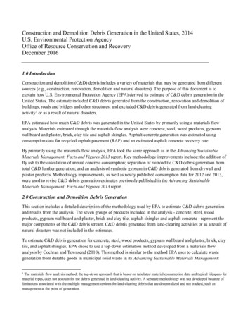
Construction and Demolition Debris Generation in the United States, 2014U.S. Environmental Protection AgencyOffice of Resource Conservation and RecoveryDecember 20161.0 IntroductionConstruction and demolition (C&D) debris includes a variety of materials that may be generated from differentsources (e.g., construction, renovation, demolition and natural disasters). The purpose of this document is toexplain how U.S. Environmental Protection Agency (EPA) derived its estimate of C&D debris generation in theUnited States. The estimate included C&D debris generated from the construction, renovation and demolition ofbuildings, roads and bridges and other structures; and excluded C&D debris generated from land-clearingactivity 1 or as a result of natural disasters.EPA estimated how much C&D debris was generated in the United States by primarily using a materials flowanalysis. Materials estimated through the materials flow analysis were concrete, steel, wood products, gypsumwallboard and plaster, brick, clay tile and asphalt shingles. Asphalt concrete generation was estimated usingconsumption data for recycled asphalt pavement (RAP) and an estimated asphalt concrete recovery rate.By primarily using the materials flow analysis, EPA took the same approach as in the Advancing SustainableMaterials Management: Facts and Figures 2013 report. Key methodology improvements include: the addition offly ash to the calculation of annual concrete consumption; separation of railroad tie C&D debris generation fromtotal C&D lumber generation; and an analysis of synthetic gypsum in C&D debris generated from drywall andplaster products. Methodology improvements, as well as newly published consumption data for 2012 and 2013,were used to revise C&D debris generation estimates previously published in the Advancing SustainableMaterials Management: Facts and Figures 2013 report.2.0 Construction and Demolition Debris GenerationThis section includes a detailed description of the methodology used by EPA to estimate C&D debris generationand results from the analysis. The seven groups of products included in the analysis - concrete, steel, woodproducts, gypsum wallboard and plaster, brick and clay tile, asphalt shingles and asphalt concrete - represent themajor components of the C&D debris stream. C&D debris generated from land-clearing activities or as a result ofnatural disasters was not included in the estimates.To estimate C&D debris generation for concrete, steel, wood products, gypsum wallboard and plaster, brick, claytile, and asphalt shingles, EPA chose to use a top-down estimation method developed from a materials flowanalysis by Cochran and Townsend (2010). This method is similar to the method EPA uses to calculate wastegeneration from durable goods in municipal solid waste in its Advancing Sustainable Materials Management:The materials flow analysis method, the top-down approach that is based on tabulated material consumption data and typical lifespans formaterial types, does not account for the debris generated in land-clearing activity. A separate methodology was not developed because oflimitations associated with the multiple management options for land-clearing debris that are decentralized and not tracked, such asmanagement at the point of generation.1
December 2016Page 2 of 23Facts and Figures reports. The materials flow method draws on publicly available historical materials-usage(consumption) data from several government and industry organizations, such as the U.S. Geological Survey(USGS) or U.S. Forest Service (USFS). Historical construction-material consumption is tabulated and typicallifespans of material types are assumed. The materials flow analysis estimates when each material has reached itsend-of-life (EOL) and is ready for management.Asphalt concrete generation was estimated using a different method. For asphalt concrete, EPA used an estimatedasphalt concrete recovery rate and data on RAP consumption published by the National Asphalt PavementAssociation (NAPA) and the U.S. Department of Transportation Federal Highway Administration (FHWA). TheRAP data are directly related to total asphalt concrete waste generation, and no assumptions about the lifespan ofasphalt concrete were required.2.1 C&D Debris Generation MethodologyBased on the Cochran and Townsend methodology, EPA derived total C&D debris generation from the sum ofwaste generated during construction and demolition activities. Figure 1 depicts the flow of materials resultingfrom construction, renovation, and demolition over the lifetime of a building, road, bridge or other structure.Cochran and Townsend define C&D debris generated during construction (C w ) as the portion of purchasedconstruction materials that are not incorporated into the actual structure, such as scraps and surplus materials.New construction and the installation phase of renovation projects both contribute to waste generated duringconstruction. All of the materials (M) are consumed in construction (M C ) or renovation (M R ) becoming part ofthe structures that will eventually be demolished. Demolition waste (D w ) is the sum of materials removed from astructure during renovation and the materials generated from a structure’s final demolition.Figure 1. Materials Flow Diagram for Construction, Renovation, and DemolitionSource: Cochran and Townsend (2010)Construction guides, used by builders to estimate the amount of materials to purchase for a construction project,provide the average amount of waste expected during construction for a range of materials. Cochran andTownsend used these guides to estimate the average percentage of materials discarded during construction, shownin Table 1. Equation 1 below shows the calculation of waste during construction for a given year based on annualmaterial consumption and average percentage of material waste during construction.
December 2016Page 3 of 23(1) C w,y M y W cwhere:C w,y amount of material waste discarded during construction in year y;M y the amount of a given material consumed in the U.S. in year y; and,W c the percentage of material discarded during new construction or the installation phase ofrenovation.Table 1. Percent of Material Discarded During ConstructionMaterialConcretePercent Discarded3%Wood ProductsDrywall and PlastersSteelBrick and Clay Tile5%10%0%4%Asphalt Shingles10%Asphalt Concrete0%Source: DelPico (2004) and Thomas (1991)Any material incorporated into the actual structure remains until removed during renovation or demolition, atwhich point it becomes demolition waste. 2 Since C&D debris generated from demolition in a given year wasdependent on the lifespan of each construction material, Cochran and Townsend (2010) calculated a range ofC&D debris generation from demolition based on the short, typical and long lifespan of the material and source ofC&D debris shown in Table 2, resulting in three different values for C&D demolition debris for each year bymaterial and source.Table 2. Lifespan of Construction Materials by Source ds & BridgesOther rBuildings5075100Railroad TiesOther Structures203545Plywood and VeneersBuildings5075100Wood PanelingDrywall and PlastersSteelBrickClay Floor & Wall TileBuildingsBuildingsBuildings/ Roads & 0010025Asphalt ShinglesBuildings202530Similarly as in Cochran and Townsend (2010), for a material such as asphalt shingles that reaches its assumed end of life before othermaterials associated with the same structure, EPA assumed that the material was removed from service through renovation, and it wasaccounted for in the demolition amount.
December 2016Page 4 of 23Table 2. Lifespan of Construction Materials by Source (years)LifespanMaterialAsphalt es: Zapata and Gambatese (2005), Katz (2004), Park et al. (2003), Scheuer et al. (2003), Junnila and Horvath (2003),Chapman and Izzo (2002), Cross and Parsons (2002), Thormark (2002), Keoleian et al. (2001), Horvath and Hendrickson(1998), Bolt (1997), and Packard (1994), Bolin and Smith (2010) (2013). Additional corroboration with USGS (2010).Table 3 shows the results for C&D debris generation of brick when using the Cochran and Townsend method forcalculating demolition debris. While this method reflects the variability in demolition debris due to theuncertainty in material lifespan, each of the three demolition waste estimates were based on a single data point,i.e., historical consumption data for a single year. Furthermore, to provide a clearer depiction in the variance ofthe total amount using this method, the overall C&D debris generation was presented as a range. However, asingle representative total waste value may be more useful to policymakers. To calculate a single representativetotal waste value for each material and source in a given year, only one demolition debris estimate must bechosen. However, it is not clear which of the three demolition debris estimates (short, typical, or long) would bethe most representative of actual demolition debris generated in a given year.Table 3 reveals that the demolition debris estimate for bricks calculated with the Cochran and Townsend methodusing the typical 75-year lifespan for bricks ranged from nearly 20 million short tons in 2000 to less than threemillion short tons in 2008. Because waste generation during construction remained fairly steady and contributedless than 10 percent of total C&D debris between 2000 and 2008, demolition debris estimates drove the observedchanges. The rapid drop in demolition debris generation between 2004 and 2007 was due to falling consumptionof bricks for construction as the Great Depression began in the late 1920s. A strong economy is indicative of highconstruction activity, and demolition activity to make space for new construction often precedes it. It seemsunlikely that in 2007, at the height of the U.S. economy before the recession, demolition waste from bricks wouldbe half of what it was in 2006 and a quarter of what it was in 2005 simply because of low consumption during theGreat Depression 75 years ago. The same issues that caused highly variable C&D debris generation using atypical material lifespan can also affect demolition debris estimates using short or long lifespans.Table 3. U.S. Annual C&D Brick Debris Generation Using Cochran and Townsend’s (2010) Methodto Calculate Demolition Debris Generation (tons)Demolition BrickLong LifeTotal C&D Brick DebrisTypicalShort LifeLifeLong 1YearBrick 8,8812002Short LifeTypical Life
December 2016Page 5 of 23Table 3. U.S. Annual C&D Brick Debris Generation Using Cochran and Townsend’s (2010) Methodto Calculate Demolition Debris Generation (tons)Demolition BrickLong LifeTotal C&D Brick DebrisTypicalShort LifeLifeLong 30915,325,7429,284,27615,498,905YearBrick 9,5722011Short LifeTypical LifeInstead of calculating demolition debris generation based on one service life at a time (short, typical, long), EPAcalculated an average demolition debris generation for the full range of years within each material’s expectedlifespan. The demolition debris generation from brick in 2014 was used as an example. The expected lifespan ofbrick ranged from 50-100 years (Table 2). EPA calculated demolition debris resulting from consumption of bricksfor each year in 1914-1964, and then averaged the results. Equation 2 below shows the calculation used toestimate demolition waste for a given year.(2) 𝐷𝐷𝑤𝑤,𝑦𝑦 (𝑦𝑦 𝑠𝑠) 𝑖𝑖 (𝑦𝑦 𝑙𝑙) (𝑀𝑀𝑖𝑖 𝐶𝐶𝑤𝑤,𝑖𝑖 )where:(𝑙𝑙 𝑠𝑠) 1y the given year for which demolition waste generation is calculated;l the longest expected lifetime of the material (see Table Y);s the shortest expected lifetime of the material;D w,y the amount of demolition waste generated from material removed during renovation ordemolition in year y;M i the amount of a given material consumed in the U.S. in year i, where i ranges from year y-l toyear y-s;C w,i the amount of material wasted during construction in year i, where i ranges from year y-l toyear y-s.Table 4 shows waste generated during construction, demolition, and total C&D debris from bricks for 2000-2014using this averaging method. The total C&D debris estimates using EPA’s method were much less susceptible tothe influence of a single historical year’s construction and consumption activity. Figure 2 shows total C&D brickdebris generated between 2000 and 2014 using EPA’s method to estimate demolition debris compared to theCochran and Townsend method.
December 2016Page 6 of 23Table 4. U.S. Annual C&D Debris Generation from Bricks Using AverageDemolition Debris Generation over the Range of Material’s Useful Life (tons)YearWaste Brick DuringConstructionDemolition BrickTotal C&D 83,59711,161,28211,344,879Figure 2. Comparison of Total C&D Debris Generation for BricksEPA’s Average Demolition Method* and Cochran and Townsend’s Short, Typicaland Long Material Lifespan method25,000,000Total Waste Short LifeShort tons20,000,00015,000,00010,000,0005,000,0000*Total C&D Debris – Average Demolition estimates shown in Table 4.Total Waste Typical LifeTotal Waste Long LifeTotal C&DDebris AverageDemolition
December 2016Page 7 of 232.2 Historical Consumption DataThe following seven sections describe the historical consumption data used for each construction material, andany assumptions necessary to determine the share of consumption associated with the construction of buildings,roads and other structures.ConcreteIn the methodology developed to estimate C&D debris generation in 2014, C&D concrete represents concretemade using either portland cement or a mix of portland cement and fly ash for cementitious material. Themethodology used to estimate concrete consumption in the Advancing Sustainable Materials Management: Factsand Figures 2013 report did not account for the use of fly ash. This year’s addition of fly ash use improves theapproximation of the overall amount of cementitious materials used in the manufacturing of concrete, which inturn, improves the accuracy of concrete consumption and generation estimates.EPA started to derive historical concrete consumption based on cement consumption data published by the USGSfor the years 1900 to 2014 (USGS, 2014a) (van Oss, 2015a and 2015b). The USGS also reports the amount ofcement, including portland cement for 1975-2013 (USGS, 2005) (van Oss, 2015b). Since cement consumptionstatistics were not readily available for years prior to 1975, EPA assumed 96 percent of cement was portlandcement, based on the data for 1975-2013. For 2014, EPA assumed the same percentage of portland cement as in2013. In addition to portland cement consumption, EPA also converted fly ash consumption to concreteconsumption. EPA used data on fly ash purchased for use in concrete and concrete products published by theAmerican Coal Ash Association for the years 2000 to 2014 (ACAA, 2015). 3 EPA used these same sources to addfly ash consumption to portland cement consumption for 2012 and 2013 and re-estimate the total C&D debrisgeneration from concrete for 2012 and 2013, resulting in increases in concrete C&D debris for both years.Although the possibility of substituting fly ash for portland cement in concrete has been known since the early1900s, fly ash was not incorporated into concrete in large quantities until the 1950s (Thomas, 2007). Fly ash mayreplace portland cement at rates ranging from 15 to 40 percent by mass, depending on the composition of the flyash and the type of construction in which the fly ash concrete will be used (EPA, 2014). In 2000, fly ashpurchased by concrete producers made up 8.2 percent of total cementitious material input. A stepwise increase of0.16 percent from zero percent in 1949 to eight percent in 1999 was used to estimate the amount of fly ash usedby concrete producers from 1950 to 1999 (see Figure 3).EPA converted portland cement and fly ash consumption into estimated concrete consumption using the densityof cement and concrete and amount of cement and fly ash used per unit of concrete. Because fly ash is asupplementary cementitious material, it is substituted one to one for portland cement on a mass basis (van Oss,2016). As cited by Cochran and Townsend (2010), the 2003 American Society for Testing Materials (ASTM)International standard reported an average density of 2,300 kg/m3 for concrete, and the Portland CementAssociation (PCA) gave an average density of 3,150 kg/m3 for portland cement and a typical concrete3U.S. cement and concrete producers purchase fly ash from coal-fired power plants to blend with cement. Most fly ash is purchaseddirectly by concrete producers instead of cement producers. USGS historical cement consumption data only include data from cementproducers (Thomas, 2007).Therefore, most of the fly ash consumed in concrete will not be captured using the USGS data on its own.
December 2016Page 8 of 23composition of 11 percent portland cement by volume. These values translated to 6.64 tons of concrete consumedper ton of portland cement. 4Figure 3. Fly Ash Purchased by Concrete Producers, 1950-201416Million Short 130EstimatedData from ACAAEPA used the method suggested by Cochran and Townsend (2010) to allocate consumption of concrete across thethree sources of concrete C&D debris: buildings, roads and bridges and other structures. PCA estimated that in2002, 47 percent of portland cement was used in buildings, 33 percent in roads and bridges, and 20 percent inother structures (Townsend and Cochran, 2010). Since this study assumes concrete consumption is directly relatedto cement consumption, the 2002 percentages for cement were used to calculate concrete consumption bybuildings, roads and bridges and other structures in 2002. The following list describes the steps taken to estimatethe division of concrete consumption among buildings, roads and bridges and other structures using the ratio fromPCA and historical datasets from the U.S. Census Bureau on the annual value of construction put-in-place 5grouped by type of structure (U.S. Census Bureau, 1975a, 1975b, 2003, 2016a, and 2016b). EPA used differencesin construction spending between 2002 and a given year in each of the three source categories to adjust the 2002percentages from PCA to reflect changes in the distribution of concrete consumption between buildings, roadsand bridges and other structures over time.1. Converted all construction put-in-place values into 1996 constant dollars:a. 1964-2002 values (U.S. Census Bureau, 2003a): No conversion necessary.b. 1915-1963 values (U.S. Census Bureau, 1975a): Converted values presented in 1957-1979constant dollars by multiplying each value by a factor of 6.39, which was the relative value of aconstant 1996 dollar to constant 1957-1959 dollar based on index tables. This value wascomputed by 1) calculating the ratio of the 1970 index value and 1957-1959 index value usingdata from series N1 and N30 (U.S. Census Bureau, 1975a); 2) calculating the ratio of the 19964Although cement and concrete density values do not consider the addition of fly ash, in the absence of a more relevant factor, EPA usedthe same 6.64 portland cement-to-concrete ratio to convert the fly ash consumption to concrete consumption.5Value of construction put-in-place represents the total dollar value of construction work done in the U.S.
December 2016Page 9 of 23index value to the 1970 index value in the 1964-2002 historical value of construction put-in-place(U.S. Census Bureau, 2003a and 2003b); and 3) multiplying these two ratios together.c. For 2003-2014 values (U.S. Census Bureau, 2008 and 2015a): Converted values presented incurrent dollars using the annual price indexes of new single-family homes (U.S. Census Bureau,2016c). The index for each year was calculated by multiplying the current dollar for a given yearby the 1996 index value and dividing by the index value of the given year.2. Calculated construction put-in-place for buildings, roads, and other structures by summation ofsubcategory values (in constant 1996 dollars).a. For 1915-2002, the buildings category included residential and non-residential buildings fromprivate and public construction as well as non-residential farm construction; roads includespublicly constructed highways, roads, and streets; and other structures includes all privatelyconstructed public utilities and all other private structures as well as public construction ofmilitary facilities, sewer and water systems, conservation and development, public serviceenterprises and all other public structures.b. For 2003-2014, the buildings category included residential and non-residential lodging, office,commercial, health care, educational, religious, public safety and amusement and recreationcategories; roads includes the highways and streets category; and other structures includes thecommunication, power, transportation, sewer and waste disposal, water supply, conservation anddevelopment and manufacturing categories.3. Calculated the ratio of spending to tons of concrete (constant 1996 dollars/ ton) consumed for buildings,roads and bridges and other structures in 2002.a. Multiplied total concrete consumption in 2002 by PCA’s estimated distribution of cement amongthe three sources in 2002 (47 percent for buildings, 33 percent for roads and bridges and 20percent for other).b. Divided 2002 construction put-in-place values for buildings, roads and bridges and otherstructures (in constant 1996 dollars) by tons of concrete consumed by each of the three categories.4. Calculated the percent of concrete use by source for each year using the spending per ton of concreteratios developed in Step 3.a. Divided spending (in constant 1996 dollars) on buildings, roads and bridges, other structures andtotal construction spending for each year by the corresponding 2002 spending per ton of concreteratio for each source.b. Divided the tons of concrete for each source estimated in Step 4a using 2002 spending ratios bythe total tons of concrete for that year derived from construction spending to calculate percentdistribution of concrete consumption across buildings, roads and bridges and other structures forthe years 1915-2014.c. Estimated 1900-1914 concrete consumption distribution for the three sources based on theaverage distribution for 1915-2014.5. Calculated the tons of concrete consumed for buildings, roads and bridges and other structures in a givenyear by multiplying the total tons of concrete consumed in construction (based on USGS cement
December 2016Page 10 of 23consumption data) by the percent distribution of concrete use associated with each source (Step 4) for agiven year.Note that revisions were made in the distribution of concrete consumption in the three C&D debris sourcecategories for 2003 through 2013 due to changes in Value of Construction Put-in-Place data published by the U.S.Census Bureau for those years.The revisions made to the distribution of concrete consumption across the three source categories; updates to the2012 and 2013 portland cement consumption data published by USGS (2015); and the methodology developedthis year to include fly ash in the calculation of concrete consumption, resulted in revised concrete generationestimates from previously published in EPA’s Advancing Sustainable Materials Management: Facts and Figures2013. The total concrete generation estimates in the previously published report of 348.449 million tons in 2012and 352.871 million tons in 2013 were revised to 364.394 million tons in 2012 and 369.542 million tons in 2013.Wood ProductsThe USGS published consumption data from the USFS for lumber, wood paneling, and plywood and veneerproducts available for 1900 to 2011 (USGS, 2014b). The USFS provided additional data for 2012 and 2013(Howard and Jones, 2016) as well as preliminary data for 2014 (Howard, 2016). EPA assumed that all woodpanels as well as plywood and veneer are used in building applications. For lumber, EPA relied on the studypublished by the USFS reporting approximately 78 percent of lumber use for construction (Howard, 2007). 6 EPAsplit that amount between buildings and railroad ties and calculated C&D lumber generation per those twosources. Namely, lumber consumed for construction of buildings was calculated by subtracting the amount ofwood used for railroad ties from total lumber used in construction.Consumption of lumber for railroad ties was based on data for annual rail tie installations from the Rail TieAssociation (RTA 2014 and 2015) (Gauntt, 2012, 2013, and 2014) and conversions associated with the use ofwood in rail ties. Data were available for the number of ties installed for Class 1 railroads from 1921 through2014 and for short line and regional railroads from 2011 through 2014. EPA assumed an annual installation rateof six million ties for the years 1900 through 1920 based on the average number of new ties installed from 1921 to1930. Data for switch and bridge ties included annual board footage for 1995 through 2014.To calculate the weight of wood consumed annually from the number of ties installed and the board footage ofswitch and bridge ties, EPA used standard conversion factors. According to the Rail Tie Association, a typical tieis seven inches tall by nine inches wide by 8.5 feet long, which is equivalent to 3.72 cubic feet per tie. Reportedboard footage for switch and bridge ties was converted to cubic feet by dividing by 12. EPA used a factor of 20.2short tons/1000 cubic feet of ties based on USFS volume-to-weight conversion factors for hardwood lumber fromUSFS (1990).Construction waste associated with the installation of ties was estimated to be five percent of annual consumption;the same rate that was used to estimate the amount of other wood products discarded during construction. ToThe remaining 22 percent of lumber is used in non-construction applications including transport packaging such as pallets andmanufacturing wooden consumer goods such as furniture (Howard, 2007).6
December 2016Page 11 of 23estimate demolition waste, railroad ties were assumed to have a lifespan ranging from 20 to 45 years with anaverage useful life of 35 years (Bolin and Smith, 2010 and 2013).The updated consumption data from USFS for 2012 and 2013, as well as the new methodology developed toestimate C&D debris generation for railroad ties, resulted in the revision of generation estimates previouslypublished in EPA’s Advancing Sustainable Materials Management: Facts and Figures 2013 for lumber, woodpaneling and plywood and veneer products. The total wood products generation estimates in the previouslypublished report of 39.968 million tons in 2012 and 40.217 million tons in 2013 were revised to 37.664 milliontons in 2012 and 38.172 million tons in 2013.Gypsum Drywall and PlastersEPA used USGS historical consumption data for gypsum for 1900 through 2014 (USGS, 2014c) (Crangle, 2015aand 2015b). USGS also published end-use statistics for gypsum, available for 1975-2013, which documentedannual consumption of drywall (listed as prefabricated products) and plasters made from calcined gypsum(USGS, 2005b) (Crangle, 2015b). EPA used these data to calculate the percent of gypsum consumed by drywalland plasters for the years 1975-2013. To calculate annual drywall and plaster consumption before 1975, EPAmultiplied total apparent gypsum consumed each year in 1900-1974 by 75 percent, the average percent of gypsumused in drywall and plasters during 1975-2012. EPA assumed the same percent of gypsum used in drywall andplasters for 2014 as calculated for 2013.Over the last two decades, an increasing amount of gypsum used in construction products has been syntheticallyproduced as a byproduct of emissions control devices at coal-fired power plants. As shown in Figure 4, theGypsum Association tracks and publishes the amount of synthetic gypsum, also known as flue gasdesulphurization (FGD) gypsum, as a percent of total gypsum used in wallboard (Gypsum Association, 2015). Asshown in Figure 4, the percent of synthetic gypsum used in wallboard was less than five percent in 1995. Theshort lifespan for drywall and plaster products was estimated to be 25 years (Table 2), which results in 1989 beingthe most recent consumption data point co
Figure 1. Materials Flow Diagram for Construction, Renovation, and Demolition . Source: Cochran and Townsend (2010) Construction guides, used by builders to estimate the amount of materials to purchase for a construction project, provide the average amount of waste expected during construction for a range of materials. Cochran and