WIXLIB

We will denote this by {x[n]}. When we have complex valued signals, sometimes we reflectand do the complex conjugation, ie, y[n] is defined by y[n]S x * [ n], where * denotes complex conjugation. This sequence will be denoted by {x *[ n]}.We will learn about more complex operations later on. Some of these operations commute,i.e. if we apply two operations we can interchange their order and some do not commute. Forexample scalar multiplication and reflection.9

2.2 SOME PROPERTIES OF SIGNALS:2.2.1 Energy of a Signal:The total enery of a signal {x[n]} is defined byA signal is reffered to as an energy signal, if and only if the total energy ofthe signal Ex is finite. An energy signal has a zero power and a power signal has infiniteenergy. There are signals which are neither energy signals nor power signals. For example{x[n]} defined by x[n] n does not have finite power or energy2.2.2 Power of a signal:If {x[n]} is a signal whose energy is not finite, we define power of the signal10

2.2.3 Periodic Signals:An important class of signals that we encounter frequently is the class of periodic signals. Wesay that a signal {x[n]} is periodic period N, where N is a positive integer, if the signal isunchanged by the time shift of N ie.,Generalizing this we get {x[n]} {x[n kN]}, where k is a positive integer. From this we seethat {x[n]} is periodic with 2N, 3N, . The fundamental period N0 isthe smallest positive value N for which the signal is periodic. The signal illustrated below isperiodic with fundamental period N0 4. {x[n]} By change of variable we can write {x[n]} {x[n N]} as {x[m N]} {x[m]} and then we see thatfor all integer values of k, positive, negative or zero. By definition, period ofa signal is always a positive integer n. Except for a all zero signal all periodic signals haveinfinite energy. They may have finite power. Let {x[n]} be periodic with period N, then thepower Px is given by11

2.2.4 Even and odd signals:A real valued signal {x[n]} is referred as an even signal if it is identical to its time reversedcounterpart ie, if {x[n]} {x[ n]} A real signal is referred to as an odd signal if {x[n]} { x[ n]} An odd signal has value 0 at n 0 as x[0] x[n] x[0]12

The signal {x[n]} is called the even part of {x[n]}. We can verify very easily that {xe[n]} is aneven signal. Similarly, {x0[n]} is called the odd part of {x[n]} and is an odd signal. When wehave complex valued signals we use a slightly different terminology. A complex valuedsignal {x[n]} is referred to as a conjugate symmetric signal if {x[n]} {x*[ n], wherex*refers to the complex conjugate of x.Here we do reflection and comple conjugation. If{x[n]} is real valuedthis is same as an even signal. A complex signal {x[n]} is referred to as aconjugate antisymmetric signal if {x[n]} { x*[ n]}. We can express any complexvalued signal as sum conjugate symmetric and conjugate antisymmetric signals. We usenotation similar to above Ev({x[n]}) {xe[n]} {1/2(x[n] x*[ n])} and Od({x[n]}) {x0[n]} {1/2(x[n] x [ n])} the {x[n]} {xe[n]} {xo[n]}. We can see easily that {xe[n]} isconjugate symmetric signal and {xo[n]} is conjugate antisymmetric signal. These definitionsreduce to even and odd signals in case signals takes only real values.2.3 PERIODICITY PROPERTIES OF SINUSOIDAL SIGNALSLet us consider the signal {x[n]} {cosw0n}. We see that if we replace w0 by (w0 2π) weget the same signal. In fact the signal with frequency w0}2π ,w0}4π and so on. This situationis quite different from continuous time signal {cosw0t, t } where each frequency isdifferent. Thus in discrete time we need to consider frequency interval of length 2π only. Aswe increase w; 0 to π signal oscillates more and more rapidly. But if we further increasefrequency from π to 2π the rate of oscillations decreases. This can be seen easily by plottingsignal cosw0n} for several values of w0. The signal {cosw0n} is not periodic for every value ofw0. For the signal to be periodic with period N 0, we should haveThus signal {cosw0n} is periodic if and only if w0 2π is a rational number. Aboveobservations also hold for complex exponential signal {x[n]} {ejw0n}2.3.1.Discrete-Time SystemsA discrete-time system can be thought of as a transformation or operator that maps an inputsequence {x[n]} to an output sequence {y[n]}By placing various conditions on T(・) we can define different classes of systems.13

3.BASIC SYSTEM PROPERTIES3.1Systems with or without memory:A system is said to be memory less if the out put for each value of the independent variable ata given time n depends only on the input value at time (t) For example system specified bythe relationship y[n] cos(x[n]) z is memory less. A particularly simple memory lesssystem is the identity system defined by y[n] x[n] In general we can write input-outputrelationship for memory less system as y[n] g(x[n]). Not all systems are memory less. Asimple example of system with memory is a delay defined by y[n] x[n 1] A system withmemory retains or stores information about input values at times other than the current inputvalue.3.2 InevitabilityA system is said to be invertible if the input signal {x[n]} can be recovered from the outputsignal {y[n]}. For this to be true two different input signals should produce two differentoutputs. If some different input signal produce same output signal then by processing outputwe can not say which input produced the output. Example of an invertible system is14

That is the system produces an all zero sequence for any input sequence. Since every inputsequence gives all zero sequence, we can not find out which input produced the output. Thesystem which produces the sequence {x[n]} from sequence {y[n]} is called the inverse system.In communication system, decoder is an inverse of the encoder.3.3 CausalityA system is causal if the output at anytime depends only on values of the input at the presenttime and in the past. y[n] f(x[n], x[n 1], .). All memory less systems are causal. Anaccumulator system defined byFor real time system where n actually denoted time causalities is important. Causality is notan essential constraint in applications where n is not time, for example, image processing. Ifwe case doing processing on recorded data, then also causality may not be required.3.4 StabilityThere are several definitions for stability. Here we will consider bounded input bondedoutput(BIBO) stability. A system is said to be BIBO stable if every bounded input produces abounded output. We say that a signal {x[n]} is bounded if15

3.5 Time invarianceA system is said to be time invariant if the behaviour and characteristics of the system do notchange with time. Thus a system is said to be time invariant if a time delay or time advance inthe input signal leads to identical delay or advance in the output signal. Mathematically if16

and so the system is not time-invariant. It is time varying. We can also see this by giving acounter example. Suppose input is {x[n]} {δ[n]} then output is allzero sequence. If the inputis {δ[n 1]} then output is {δ[n 1]} which is definitely not a shifted version version of allzero sequence.3.6 LinearityThis is an important property of the system. We will see later that if we have system which islinear and time invariant then it has a very compact representation. A linear system possessesthe important property of super position: if an input consists of weighted sum of severalsignals, the output is also weighted sum of the responses of the system to each of those inputsignals. Mathematically let {y1[n]} be the response of the system to the input {x1[n]} and let{y2[n]} be the response of the system to the input {x2[n]}. Then the system is linear if:1. Additivity: The response to {x1[n]} {x2[n]} is {y1[n]} {y2[n]}2. Homogeneity: The response to a{x1[n]} is a{y1[n]}, where a is any real number if we areconsidering only real signals and a is any complex number if we are considering complexvalued signals.3. Continuity: Let us consider {x1[n]}, {x2[n]}, .{xk[n]}. be countably infinite number ofsignals such that lim{ xk[n]} {x[n]} Let the corresponding output signals be denoted by{yn[n]} k and Lim { yn[n]} {y[n]} We say that system processes the continuity propertyk if the response of the system to the limiting input {x[n]} is limit of the responses {y[n]}.T( lim{ xk[n]}) lim T({Xk[n]}) k k The additive and continuity properties can be replaced by requiring that We say that systemposseses the continuity property system is additive for countably infinite number if signalsi.e. response to{x1[n]} {x2[n]} . {xn[n]} . is {y1[n]} {y2[n]} . {yk[n]} .Most of thebooks do not mention the continuity property. They state only finite additivity andhomogeneity. But from finite additivity we can not deduce c. additivity. This distinctionbecomes very important in continuous time systems. A system can be linear without beingtime invariant and it can be time invariant without being linear. If a system is linear, an allzero input sequence will produce a all zero output sequence. {0} denote the all zero sequence,then {0} 0.{x[n]}.If T({x[n]} {y[n]}) then by homogeneity property T(0.{x[n]}) 0.{y[n]}T({0}) {0}Consider the system defined byy[n] 2x[n] 3This system is not linear. This can be verified in several ways. If the input is all zerosequence {0}, the output is not an all zero sequence. Although the defining equation is alinear equation is x and y the system is nonlinear. The output of this system can berepresented as sum of a linear system and another signal equal to the zero input response. Inthis case the linear system is y[n] 2x[n] and the zero-input response is y0[n] 3 for all n17

systems correspond to the class of incrementally linear system. System is linear in term ofdifference signal i.e if we define {xd[n]} {x1[n]} {X2[n]}and {yd[n]} {y1[n]} {y2[n]}.Then in terms of {xd[n]} and {yd[n]} the system is linear.4. MODELS OF THE DISCRETE-TIME SYSTEMFirst let us consider a discrete-time system as an interconnection of only three basiccomponents: the delay elements, multipliers, and adders. The input– output relationships forthese components and their symbols are shown in Figure below. The fourth component is themodulator, which multiplies two or more signals and hence performs a nonlinear operation.The basic components used in a discrete-time system18

simple discrete-time system is shown in Figure 5, where input signal x(n) {x(0), x(1), x(2),x(3)} is shown to the left of v0(n) x(n). The signal v1(n)shown on the left is the signalx(n)delayed by T seconds or one sample, so, v1(n) x(n 1). Similarly, v(2)and v(3)are thesignals obtained from x(n)when it is delayed by 2T and 3T seconds: v2(n) x(n 2)and v3(n) x(n 3). When we say that the signal x(n)is delayed by T, 2T , or 3T seconds, we mean thatthe samples of the sequence are present T, 2T, or 3T seconds later, as shown by the plots ofthe signals to the left of v1(n), v2(n), and v3(n). But at any given time t nT , the samples inv1(n), v2(n), and v3(n) are the samples of the input signal that occur T,2T , and 3T secondsprevious to t nT . For example, at t 3T , the value of the sample in x(n)is x(3), and thevalues present in v1(n), v2(n)and v3(n)are x(2), x(1), and x(0) respectively.Agoodunderstanding of the operation of the discrete-time system as illustrated in above Figure isessential in analyzing, testing, and debugging the operation of the system when availablesoftware is used for the design, simulation, and hardware implementation of the system.It is easily seen that the output signal in above Figure iswhere b(0), b(1), b(2), b(3)are the gain constants of the multipliers. It is also easy to see fromthe last expression that the output signal is the weighted sum of the current value and theprevious three values of the input signal. So this gives us an input–output relationship for thesystem shown in belowOperations in a typical discrete-time system19

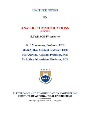
Now we consider another example of a discrete-time system, shown in Figure 5. Note that afundamental rule is to express the output of the adders and generate as many equations as thenumber of adders found in this circuit diagram for the discrete-time system. (This step issimilar to writing the node equations for an analog electric circuit.) Denoting the outputs ofthe three adders as y1(n), y2(n), and y3(n), we getSchematic circuit for a discrete-time system.20

These three equations give us a mathematical model derived from the model shown in abovethat is schematic in nature. We can also derive (draw the circuit realization) the model shownin Figure 5 from the same equations given above. After eliminating the internal variablesy1(n)and y2(n); that relationship constitutes the third model for the system. The general formof such an input– output relationship isEq(1)or in another equivalent formEq(1) shows that the output y(n)is determined by the weighted sum of the previous N valuesof the output and the weighted sum of the current and previous M 1 values of the input.Very often the coefficient a(0)as shown in Eq(2) is normalized to unity.5. LINEAR TIME-INVARIANT, CAUSAL SYSTEMSIn this section, we study linear time-invariant causal systems and focus on properties such aslinearity, time invariance, and causality.5.1 Linearity:A linear system is illustrated in below figure, where y1(n) is the system output using an inputx1(n), and y2(n) is the system output using an input x2(n). This Figure illustrates that thesystem output due to the weighted sum inputs αx1(n) βx2(n) is equal to the same weightedsum of the individual outputs obtained from their corresponding inputs, that isy(n) αy1(n) βy2(n)where α and β are constants.For example, assuming a digital amplifier as y(n) 10x(n), the input is multiplied by 10 togenerate the output. The inputs x1(n) u(n) and x2(n) δ(n) generate the outputs y1(n) 10u(n) and y2(n) 10δ(n), respectively. If, as described in below Figure , we apply to thesystem using the combined input x(n), where the first input is multiplied by a constant 2while the second input is multiplied by a constant 4, x(n) 2x1(n) 4x2(n) 2u(n) 4δ(n),21

5.2 Time InvarianceA time-invariant system is illustrated in Figure below, where y1(n) is the system output forthe input x1(n). Let x2(n) x1(n - n0) be the shifted version of x1(n)by n0 samples. The output y2(n) obtained with the shifted input x2(n) x1(n - n0)is equivalentto the output y2(n) acquired by shifting y1(n) by n0 samples,y2(n) y1(n - n0).This can simplybe viewed as the following. If the system is time invariant and y1(n) is the system output dueto the input x1(n),then the shifted system input x1(n -n0) will produce a shifted system outputy1(n - n0)by the same amount of time n0.5.3 Differential Equations and Impulse Responses:A causal, linear, time-invariant system can be described by a difference equation having thefollowing general form:y(n) a1y(n - 1) . . . aNy(n - N) b0x(n) b1x(n -1) . . . bMx(n -M) where a1, . . . , aNand b0, b1, . . . , bM are the coefficients of the difference equation. It can further be written asy(n) - a1y(n - 1) -. . . - aNy(n - N) b0x(n) b1x(n - 1) . . . bMx(n -M)1. FOURIER SERIES COEFFICIENTS OF PERIODIC IN DIGITAL SIGNALS:22

Let us look at a process in which we want to estimate the spectrum of a periodic digital signalx(n) sampled at a rate of fs Hz with the fundamental period T0 NT, as shown in below, wherethere are N samples within the duration of the fundamental period and T 1/fs is thesampling period. For the time being, we assume that the periodic digital signal is band limitedto have all harmonic frequencies less than the folding frequency fs 2 so that aliasing does notoccur. According to Fourier series analysis (Appendix B), the coefficients of the Fourierseries expansion of a periodic signal x(t) in a complex form isTherefore, the two-sided line amplitude spectrum jckj is periodic, as shown inFigure 4.3. We note the following points:a. As displayed in Figure 4.3, only the line spectral portion between the frequency fs 2 andfrequency fs 2 (folding frequency) represents the frequency information of the periodicsignal.23

b. Notice that the spectral portion from fs 2 to fs is a copy of the spectrum in the negativefrequency range from fs 2 to 0 Hz due to the spectrum being periodic for every Nf 0 Hz.Again, the amplitude spectral components indexed from fs 2 to fs can be folded at thefolding frequency fs 2 to match the amplitude spectral components indexed from 0 to fs 2 interms of fs f Hz, where f is in the range from fs 2 to fs. For convenience, we compute thespectrum over the range from 0 to fs Hz with nonnegative indices, that is,c. For the kth harmonic, the frequency is f kf0 Hz. The frequency spacing between theconsecutive spectral lines, called the frequency resolution, is f0 Hz7. Discrete Fourier TransformNow, let us concentrate on development of the DFT. In below Figure shows one way toobtain the DFT formula. First, we assume that the process acquires data samples fromdigitizing the interested continuous signal for a duration of T seconds. Next, we assume that aperiodic signal x(n) is obtained by copying the acquired N data samples with the duration ofT to itself repetitively. Note that we assume continuity between the N data sample frames.This is not true in practice. We will tackle this problem in Section 4.3. We determine theFourier series coefficients using one-period N data samples and Equation (4.5). Then wemultiply the Fourier series coefficients by a factor of N to obtainwhere X(k) constitutes the DFT coefficients. Notice that the factor of N is a constant and doesnot affect the relative magnitudes of the DFT coefficients X(k). As shown in the last plot,applying DFT with N data samples of x(n) sampled at a rate of fs (sampling period is T 1/fs) produces N complex DFT24

As we know, the spectrum in the range of -2 to 2 Hz presents the information

Also digital signal processing tries to implement this as closely as possible. Thus what we study is mostly discrete time signal processing and what is really implemented is digital signal processing. 1.3 ELEMENTARY SIGNALS There are several elementary signals that feature prominently in the study of digital signals and digital signal processing.