Transcription
COMPARISON OF DISCRETE AND CONTINUOUS WAVELETTRANSFORMSPALLE E.T. JORGENSEN AND MYUNG-SIN SONGArticle OutlineGlossary1. Definition2. Introduction3. The discrete vs continuous wavelet Algorithms3.1. The Discrete Wavelet Transform3.2. The Continuous Wavelet Transform3.3. Some background on Hilbert space3.4. Connections to group theory4. List of names and discoveries5. History6. Tools from Mathematics7. A Transfer Operator8. Future Directions9. Literature10. s glossary consists of a list of terms used inside the paper: In mathematics,in probability, in engineering, and on occasion in physics. To clarify the seeminglyconfusing use of up to four different names for the same idea or concept, we havefurther added informal explanations spelling out the reasons behind the differencesin current terminology from neighboring fields.Disclaimer: This glossary has the structure of four columns. A number of termsare listed line by line, and each line is followed by explanation. Some “terms” haveup to four separate (yet commonly accepted) tionrandom variablesignalstate(measurable)Mathematically, functions may map between any two sets, say,from X to Y ; but if X is a probability space (typically called Ω),it comes with a σ-algebra B of measurable sets, and probabilitymeasure P . Elements E in B are called events, and P(E)Work supported in part by the U.S. National Science Foundation.1
2PALLE E.T. JORGENSEN AND MYUNG-SIN SONGmathematicsprobabilityengineeringphysicsthe probability of E. Corresponding measurable functions withvalues in a vector space are called random variables, a terminologywhich suggests a stochastic viewpoint. The function values of arandom variable may represent the outcomes of an experiment,for example “throwing of a die.”Yet, function theory is widely used in engineering wherefunctions are typically thought of as signal. In this case, X maybe the real line for time, or Rd . Engineers visualize functions assignals. A particular signal may have a stochastic component,and this feature simply introduces an extra stochastic variableinto the “signal,” for example noise.Turning to physics, in our present application, the physicalfunctions will be typically be in some L2 -space, and L2 -functionswith unit norm represent quantum mechanical “states.”sequence (incl.random ally, a sequence is a function defined on the integersZ or on subsets of Z, for example the natural numbers N. Hence,if time is discrete, this to the engineer represents a time series,such as a speech signal, or any measurement which depends ontime. But we will also allow functions on lattices such as Zd .In the case d 2, we may be considering the grayscale numbers which represent exposure in a digital camera. In this case,the function (grayscale) is defined on a subset of Z2 , and is thensimply a matrix.A random walk on Zd is an assignment of a sequential andrandom motion as a function of time. The randomness presupposes assigned probabilities. But we will use the term “randomwalk” also in connection with random walks on combinatorialtrees.nestedrefinementmultiresolution scales of visualsubspacesresolutionsWhile finite or infinite families of nested subspaces are ubiquitousin mathematics, and have been popular in Hilbert space theoryfor generations (at least since the 1930s), this idea was revived ina different guise in 1986 by Stéphane Mallat, then an engineeringgraduate student. In its adaptation to wavelets, the idea is nowreferred to as the multiresolution method.What made the idea especially popular in the wavelet community was that it offered a skeleton on which various discretealgorithms in applied mathematics could be attached and turnedinto wavelet constructions in harmonic analysis. In fact what wenow call multiresolutions have come to signify a crucial link between the world of discrete wavelet algorithms, which are popularin computational mathematics and in engineering (signal/image
COMPARISON OF DISCRETE AND CONTINUOUS WAVELET TRANSFORMSprocessing, data mining, etc.) on the one side, and on the otherside continuous wavelet bases in function spaces, especially inL2 (Rd ). Further, the multiresolution idea closely mimics howfractals are analyzed with the use of finite function systems.But in mathematics, or more precisely in operator theory,the underlying idea dates back to work of John von Neumann,Norbert Wiener, and Herman Wold, where nested and closed subspaces in Hilbert space were used extensively in an axiomatic approach to stationary processes, especially for time series. Woldproved that any (stationary) time series can be decomposed intotwo different parts: The first (deterministic) part can be exactlydescribed by a linear combination of its own past, while the second part is the opposite extreme; it is unitary, in the language ofvon Neumann.von Neumann’s version of the same theorem is a pillar inoperator theory. It states that every isometry in a Hilbert spaceH is the unique sum of a shift isometry and a unitary operator,i.e., the initial Hilbert space H splits canonically as an orthogonalsum of two subspaces Hs and Hu in H, one which carries the shiftoperator, and the other Hu the unitary part. The shift isometryis defined from a nested scale of closed spaces Vn , such that theintersection of these spaces is Hu . Specifically,· · · V 1 V0 V1 V2 · · · Vn Vn 1 · · · Vn Hu , andVn H.nnHowever, Stéphane Mallat was motivated instead by the notion of scales of resolutions in the sense of optics. This in turnis based on a certain “artificial-intelligence” approach to visionand optics, developed earlier by David Marr at MIT, an approachwhich imitates the mechanism of vision in the human eye.The connection from these developments in the 1980s backto von Neumann is this: Each of the closed subspaces Vn corresponds to a level of resolution in such a way that a larger subspacerepresents a finer resolution. Resolutions are relative, not absolute! In this view, the relative complement of the smaller (orcoarser) subspace in larger space then represents the visual detailwhich is added in passing from a blurred image to a finer one, i.e.,to a finer visual resolution.This view became an instant hit in the wavelet community, as it offered a repository for the fundamental father andthe mother functions, also called the scaling function ϕ, and thewavelet function ψ. Via a system of translation and scaling operators, these functions then generate nested subspaces, and werecover the scaling identities which initialize the appropriate algorithms. What results is now called the family of pyramid algorithms in wavelet analysis. The approach itself is called themultiresolution approach (MRA) to wavelets. And in the meantime various generalizations (GMRAs) have emerged.3
4PALLE E.T. JORGENSEN AND MYUNG-SIN SONGmathematicsprobabilityengineeringphysicsIn all of this, there was a second “accident” at play: As it turnedout, pyramid algorithms in wavelet analysis now lend themselvesvia multiresolutions, or nested scales of closed subspaces, to ananalysis based on frequency bands. Here we refer to bands offrequencies as they have already been used for a long time insignal processing.One reason for the success in varied disciplines of the samegeometric idea is perhaps that it is closely modeled on how wehistorically have represented numbers in the positional numbersystem. Analogies to the Euclidean algorithm seem especiallycompelling.operatorprocessblack boxobservable(if selfadjoint)In linear algebra students are familiar with the distinctions between (linear) transformations T (here called “operators”) andmatrices. For a fixed operator T : V W , there is a variety ofmatrices, one for each choice of basis in V and in W . In manyengineering applications, the transformations are not restrictedto be linear, but instead represent some experiment (“black box,”in Norbert Wiener’s terminology), one with an input and an output, usually functions of time. The input could be an externalvoltage function, the black box an electric circuit, and the outputthe resulting voltage in the circuit. (The output is a solution toa differential equation.)This context is somewhat different from that of quantum mechanical (QM) operators T : V V where V is a Hilbert space.In QM, selfadjoint operators represent observables such as position Q and momentum P , or time and energy.Fourier dualgeneratingtime/frequency P /QpairfunctionThe following dual pairs position Q/momentum P , and time/energymay be computed with the use of Fourier series or Fourier transforms; and in this sense they are examples of Fourier dual pairs.If for example time is discrete, then frequency may be representedby numbers in the interval [ 0, 2π); or in [ 0, 1) if we enter the number 2π into the Fourier exponential. Functions of the frequencyare then periodic, so the two endpoints are identified. In the caseof the interval [ 0, 1), 0 on the left is identified with 1 on the right.So a low frequency band is an interval centered at 0, while a highfrequency band is an interval centered at 1/2. Let a function Won [ 0, 1) represent a probability assignment. Such functions Ware thought of as “filters” in signal processing. We say that W islow-pass if it is 1 at 0, or if it is near 1 for frequencies near 0.
COMPARISON OF DISCRETE AND CONTINUOUS WAVELET Low-pass filters pass signals with low frequencies, and block theothers.If instead some filter W is 1 at 1/2, or takes values near 1 forfrequencies near 1/2, then we say that W is high-pass; it passessignals with high frequency.convolution—filtersmearingPointwise multiplication of functions of frequencies correspondsin the Fourier dual time-domain to the operation of convolution(or of Cauchy product if the time-scale is discrete.) The processof modifying a signal with a fixed convolution is called a linearfilter in signal processing. The corresponding Fourier dual frequency function is then referred to as “frequency response” orthe “frequency response function.”More generally, in the continuous case, since convolutiontends to improve smoothness of functions, physicists call it .g., Fouriercomponentscoefficients in aFourier expansion)Calculating the Fourier coefficients is “analysis,” and adding upthe pure frequencies (i.e., summing the Fourier series) is calledsynthesis. But this view carries over more generally to engineering where there are more operations involved on the two sides,e.g., breaking up a signal into its frequency bands, transformingfurther, and then adding up the “banded” functions in the end.If the signal out is the same as the signal in, we say that theanalysis/synthesis yields perfect osition(e.g., inverseFourier transform)Here the terms related to “synthesis” refer to the second halfof the kind of signal-processing design outlined in the previousparagraph.subspace—resolution(signals in a)frequency bandFor a space of functions (signals), the selection of certain frequencies serves as a way of selecting special signals. When the processof scaling is introduced into optics of a digital camera, we note5
6PALLE E.T. JORGENSEN AND MYUNG-SIN SONGmathematicsprobabilityengineeringphysicsthat a nested family of subspaces corresponds to a grading of visual resolutions.Cuntz relations —perfectsubbandreconstructiondecompositionfrom subbandsN 1XSi Si 1, and Si Sj δi,j 1.i 0inner of transitionfrom one stateto anotherIn many applications, a vector space with inner product capturesperfectly the geometric and probabilistic features of the situation.This can be axiomatized in the language of Hilbert space; and theinner product is the most crucial ingredient in the familiar axiomsystem for Hilbert space.fout T fintransformationof statesSystems theory language for operators T : V W . Then vectorsin V are input, and in the range of T ly, think of a fractal as reflecting similarity of scales suchas is seen in fern-like images that look “roughly” the same atsmall and at large scales. Fractals are produced from an infiniteiteration of a finite set of maps, and this algorithm is perfectlysuited to the kind of subdivision which is a cornerstone of thediscrete wavelet algorithm. Self-similarity could refer alternatelyto space, and to time. And further versatility is added, in thatflexibility is allowed into the definition of “similar.”—data mining—The problem of how to handle and make use of large volumes ofdata is a corollary of the digital revolution. As a result, the subject of data mining itself changes rapidly. Digitized information(data) is now easy to capture automatically and to store electronically. In science, in commerce, and in industry, data representscollected observations and information: In business, there is dataon markets, competitors, and customers. In manufacturing, thereis data for optimizing production opportunities, and for improving processes. A tremendous potential for data mining exists in
COMPARISON OF DISCRETE AND CONTINUOUS WAVELET TRANSFORMS7medicine, genetics, and energy. But raw data is not always directly usable, as is evident by inspection. A key to advances isour ability to extract information and knowledge from the data(hence “data mining”), and to understand the phenomena governing data sources. Data mining is now taught in a variety of formsin engineering departments, as well as in statistics and computerscience departments.One of the structures often hidden in data sets is some degreeof scale. The goal is to detect and identify one or more naturalglobal and local scales in the data. Once this is done, it is oftenpossible to detect associated similarities of scale, much like the familiar scale-similarity from multidimensional wavelets, and fromfractals. Indeed, various adaptations of wavelet-like algorithmshave been shown to be useful. These algorithms themselves areuseful in detecting scale-similarities, and are applicable to othertypes of pattern recognition. Hence, in this context, generalizedmultiresolutions offer another tool for discovering structures inlarge data sets, such as those stored in the resources of the Internet. Because of the sheer volume of data involved, a strictly manual analysis is out of the question. Instead, sophisticated queryprocessors based on statistical and mathematical techniques areused in generating insights and extracting conclusions from datasets.Multiresolutions. Haar’s work in 1909–1910 had implicitly the key idea which gotwavelet mathematics started on a roll 75 years later with Yves Meyer, IngridDaubechies, Stéphane Mallat, and others—namely the idea of a multiresolution.In that respect Haar was ahead of his time. See Figures 1 and 2 for details.Scaling OperatorϕψW0. V-1 V0 V1 V2 V3 .Figure 1. Multiresolution. L2 (Rd )-version (continuous); ϕ V0 ,ψ W0 .2S0S1.S0S1S1S0S0Figure 2. Multiresolution. l2 (Z)-version (discrete); ϕ V0 , ψ W0 .
8PALLE E.T. JORGENSEN AND MYUNG-SIN SONG· · · V 1 V0 V1 · · · , V0 W0 V1The word “multiresolution” suggests a connection to optics from physics. Sothat should have been a hint to mathematicians to take a closer look at trendsin signal and image processing! Moreover, even staying within mathematics, itturns out that as a general notion this same idea of a “multiresolution” has longroots in mathematics, even in such modern and pure areas as operator theory andHilbert-space geometry. Looking even closer at these interconnections, we can nowrecognize scales of subspaces (so-called multiresolutions) in classical algorithmicconstruction of orthogonal bases in inner-product spaces, now taught in lots ofmathematics courses under the name of the Gram–Schmidt algorithm. Indeed, acloser look at good old Gram–Schmidt reveals that it is a matrix algorithm, Hencenew mathematical tools involving non-commutativity!If the signal to be analyzed is an image, then why not select a fixed but suitable resolution (or a subspace of signals corresponding to a selected resolution),and then do the computations there? The selection of a fixed “resolution” is dictated by practical concerns. That idea was key in turning computation of waveletcoefficients into iterated matrix algorithms. As the matrix operations get large,the computation is carried out in a variety of paths arising from big matrix products. The dichotomy, continuous vs. discrete, is quite familiar to engineers. Theindustrial engineers typically work with huge volumes of numbers.Numbers! — So why wavelets? Well, what matters to the industrial engineeris not really the wavelets, but the fact that special wavelet functions serve as anefficient way to encode large data sets—I mean encode for computations. And thewavelet algorithms are computational. They work on numbers. Encoding numbersinto pictures, images, or graphs of functions comes later, perhaps at the very end ofthe computation. But without the graphics, I doubt that we would understand anyof this half as well as we do now. The same can be said for the many issues thatrelate to the crucial mathematical concept of self-similarity, as we know it fromfractals, and more generally from recursive algorithms.1. DefinitionIn this paper we outline several points of view on the interplay between discreteand continuous wavelet transforms; stressing both pure and applied aspects of both.We outline some new links between the two transform technologies based on thetheory of representations of generators and relations. By this we mean a finitesystem of generators which are represented by operators in Hilbert space. Wefurther outline how these representations yield sub-band filter banks for signal andimage processing algorithms.The word “wavelet transform” (WT) means different things to different people:Pure and applied mathematicians typically give different answers the questions“What is the WT?” And engineers in turn have their own preferred quite differentapproach to WTs. Still there are two main trends in how WTs are used, thecontinuous WT on one side, and the discrete WT on the other. Here we offer auserfriendly outline of both, but with a slant toward geometric methods from thetheory of operators in Hilbert space.Our paper is organized as follows: For the benefit of diverse reader groups, webegin with Glossary (section ). This is a substantial part of our account, and itreflects the multiplicity of how the subject is used.
COMPARISON OF DISCRETE AND CONTINUOUS WAVELET TRANSFORMS9The concept of multiresolutions or multiresolution analysis (MRA) serves as alink between the discrete and continuous theory.In section 4, we summarize how different mathematicians and scientists havecontributed to and shaped the subject over the years.The next two sections then offer a technical overview of both discrete and thecontinuous WTs. This includes basic tools from Fourier analysis and from operatorsin Hilbert space. In sections 6 and 7 we outline the connections between the separateparts of mathematics and their applications to WTs.2. IntroductionWhile applied problems such as time series, signals and processing of digitalimages come from engineering and from the sciences, they have in the past twodecades taken a life of their own as an exciting new area of applied mathematics. While searches in Google on these keywords typically yield sites numbered inthe millions, the diversity of applications is wide, and it seems reasonable here tonarrow our focus to some of the approaches that are both more mathematical andmore recent. For references, see for example [1, 6, 23, 31]. In addition, our owninterests (e.g., [20, 21, 27, 28]) have colored the presentation below. Each of the twoareas, the discrete side, and the continuous theory is huge as measured by recentjournal publications. A leading theme in our article is the independent interest ina multitude of interconnections between the discrete algorithm and their uses inthe more mathematical analysis of function spaces (continuous wavelet transforms).The mathematics involved in the study and the applications of this interaction wefeel is of benefit to both mathematicians and to engineers. See also [20]. An earlypaper [9] by Daubechies and Lagarias was especially influential in connecting thetwo worlds, discrete and continuous.3. The discrete vs continuous wavelet Algorithms3.1. The Discrete Wavelet Transform. If one stays with function spaces, it isthen popular to pick the d-dimensional Lebesgue measure on Rd , d 1, 2, , andpass to the Hilbert space L2 (Rd ) of all square integrable functions on Rd , referringto d-dimensional Lebesgue measure. A wavelet basis refers to a family of basisfunctions for L2 (Rd ) generated from a finite set of normalized functions ψi , theindex i chosen from a fixed and finite index set I, and from two operations, onecalled scaling, and the other translation. The scaling is typically specified by a dby d matrix over the integers Z such that all the eigenvalues in modulus are biggerthan one, lie outside the closed unit disk in the complex plane. The d-lattice isdenoted Zd , and the translations will be by vectors selected from Zd . We say thatwe have a wavelet basis if the triple indexed family ψi,j,k (x) : detA j/2 ψ(Aj x k)forms an orthonormal basis (ONB) for L2 (Rd ) as i varies in I, j Z, and k Rd .The word “orthonormal” for a family F of vectors in a Hilbert space H refers tothe norm and the inner product in H: The vectors in an orthonormal family F areassumed to have norm one, and to be mutually orthogonal. If the family is alsototal (i.e., the vectors in F span a subspace which is dense in H), we say that F isan orthonormal basis (ONB.)While there are other popular wavelet bases, for example frame bases, and dualbases (see e.g., [2, 14] and the papers cited there), the ONBs are the most agreeableat least from the mathematical point of view.
10PALLE E.T. JORGENSEN AND MYUNG-SIN SONGThat there are bases of this kind is not at all clear, and the subject of wavelets inthis continuous context has gained much from its connections to the discrete worldof signal- and image processing.Here we shall outline some of these connections with an emphasis on the mathematical context. So we will be stressing the theory of Hilbert space, and boundedlinear operators acting in Hilbert space H, both individual operators, and familiesof operators which form algebras.As was noticed recently the operators which specify particular subband algorithms from the discrete world of signal- processing turn out to satisfy relationsthat were found (or rediscovered independently) in the theory of operator algebras,and which go under the name of Cuntz algebras, denoted ON if n is the number ofbands. For additional details, see e.g., [21]. 1In symbols the C algebra has generators (Si )Ni 0 , and the relations areN 1X(3.1)Si Si 1i 0(where 1 is the identity element in ON ) andN 1X(3.2)Si Si 1, and Si Sj δi,j 1.i 0In a representation on a Hilbert space, say H, the symbols Si turn into boundedoperators, also denoted Si , and the identity element 1 turns into the identity operator I in H, i.e., the operator I : h h, for h H. In operator language, the twoformulas 3.1 and 3.2 state that each Si is an isometry in H, and that te respectiveranges Si H are mutually orthogonal, i.e., Si H Sj H for i 6 j. Introducing theprojections Pi Si Si , we get Pi Pj δi,j Pi , andN 1XPi Ii 0In the engineering literature this takes the form of programming diagrams: u uInput u.Si * udown-sampling u.Si.ROutput uup-samplingFigure 3. Perfect reconstruction in a subband filtering as used insignal and image processing.
COMPARISON OF DISCRETE AND CONTINUOUS WAVELET TRANSFORMS11If the process of Figure 3 is repeated, we arrive at the discrete wavelet transformfirst detail levelsecond detail levelthird detail levelor stated in the form of images (n 5)S0SHSHS0SDS0SVSVSDFigure 4. The subdivided squares represent the use of the pyramid subdivision algorithm to image processing, as it is used onpixel squares. At each subdivision step the top left-hand squarerepresents averages of nearby pixel numbers, averages taken withrespect to the chosen low-pass filter; while the three directions, horizontal, vertical, and diagonal represent detail differences, with thethree represented by separate bands and filters. So in this model,there are four bands, and they may be realized by a tensor product construction applied to dyadic filters in the separate x- andthe y-directions in the plane. For the discrete WT used in imageprocessing, we use iteration of four isometries S0 , SH , SV , andSDwith mutually orthogonal ranges, and satisfying the following sum rule S0 S0 SH SH SV SV SD SD I, with I denoting the identity2operator in an appropriate l -space.
12PALLE E.T. JORGENSEN AND MYUNG-SIN SONGFigure 5. n 2 JorgensenSelecting a resolution subspace V0 closure span{ϕ(· k) k Z}, we arriveat a wavelet subdivision {ψj,k j P 0, k Z}, where ψj,k (x) 2j/2 ψ(2j x k), andthe continuous expansion f j,k hψj,k f iψj,k or the discrete analogue derivedfrom the isometries, i 1, 2, · · · , N 1, S0k Si for k 0, 1, 2, · · · ; called the discretewavelet transform.Notational convention. In algorithms, the letter N is popular, and often used forcounting more than one thing.In the present contest of the Discete Wavelet Algorithm (DWA) or DWT, wecount two things, “the number of times a picture is decomposed via subdivision”.We have used n for this. The other related but different number N is the number ofsubbands, N 2 for the dyadic DWT, and N 4 for the image DWT. The imageprocessing WT in our present context is the tensor product of the 1-D dyadicWT, so 2 2 4. Caution: Not all DWAs arise as tensor products of N 2models. The wavelets coming from tensor products are called separable. When aparticular image-processing scheme is used for generating continuous wavelets it isnot transparent if we are looking at a separable or inseparable wavelet!To clarify the distinction, it is helpful to look at the representations of the Cuntzrelations by operators in Hilbert space. We are dealing with representations of the
COMPARISON OF DISCRETE AND CONTINUOUS WAVELET TRANSFORMS13two distinct algebras O2 , and O4 ; two frequency subbands vs 4 subbands. Notethat the Cuntz O2 , and O4 are given axiomatic, or purely symbolically. It is onlywhen subband filters are chosen that we get representations. This also means thatthe choice of N is made initially; and the same N is used in different runs of theprograms. In contrast, the number of times a picture is decomposed varies fromone experiment to the next!Summary: N 2 for the dyadic DWT: The operators in the representationare S0 , S1 . One average operator, and one detail operator. The detail operator S1“counts” local detail variations.Image-processing. Then N 4 is fixed as we run different images in the DWT:The operators are now: S0 , SH , SV , SD . One average operator, and three detailoperator for local detail variations in the three directions in the plane.3.2. The Continuous Wavelet Transform. Consider functions f on the realline R. We select the Hilbert space of functions to be L2 (R) To start a continuousWT, we must select a function ψ L2 (R) and r, s R such that the followingfamily of functionsx sψr,s (x) r 1/2 ψ()rcreates an over-complete basis for L2 (R). An over-complete family of vectors ina Hilbert space is often called a coherent decomposition. This terminology comesfrom quantum optics. What is needed for a continuous WT in the simplest case isthe following representation valid for all f L2 (R):Z Zdrdsf (x) Cψ 1hψr,s f iψr,s (x) 2r2RRRdωwhere Cψ : R ψ̂(ω) 2 ω and where hψr,s f i R ψr,s (y)f (y)dy. The refinementsand implications of this are spelled out in tables in section 3.43.3. Some background on Hilbert space. Wavelet theory is the art of finding aspecial kind of basis in Hilbert space. Let H be a Hilbert space over C and denotethe inner product h · · i. For us, it is assumed linear in the second variable. IfH L2 (R), thenZh f g i : If H ℓ2 (Z), thenf (x) g (x) dx.Rh ξ η i : Let T R/2πZ. If H L2 (T), thenh f g i : 12πZXξ n ηn .n Zπf (θ) g (θ) dθ. πFunctions f L2 (T) have Fourier series: Setting en (θ) einθ ,Z π1e inθ f (θ) dθ,fˆ (n) : h en f i 2π πand2kf kL2 (T) Xn Z2fˆ (n) .
14PALLE E.T. JORGENSEN AND MYUNG-SIN SONGSimilarly if f L2 (R), thenfˆ (t) : Ze ixt f (x) dx,RandZ21 fˆ (t) dt.2π RLet J be an index set. We shall only need to consider the case when J iscountable. Let {ψα }α J be a family of nonzero vectors in a Hilbert space H. Wesay it is an orthonormal basis (ONB) if2kf kL2 (R)(3.3)h ψα ψβ i δα,βand if(3.4)Xα J(Kronecker delta) h ψα f i 2 kf k2holds for all f H.If only (3.4) is assumed, but not (3.3), we say that {ψα }α J is a (normalized) tightframe. We say that it is a frame with frame constants 0 A B ifX222A kf k h ψα f i B kf kholds for all f H.α JIntroducing the rank-one operators Qα : ψα i hψα of Dirac’s terminology, see [3],we see that {ψα }α J is an ONB if and only if the Qα ’s are projections, andX(3.5)Qα I( the identity operator in H).α JIt is a (normalized) tight frame if and only if (3.5) holds but with no furtherrestriction on the rank-one operators Qα . It is a frame with frame constants A andB if the operatorXS : Qαα JsatisfiesAI S BIin the order of hermitian operators. (We say that operators Hi Hi , i 1, 2,satisfy H1 H2 if h f H1 f i h f H2 f i holds for all f H). If h, k are vectorsin a Hilbert spa
3. The discrete vs continuous wavelet Algorithms 9 3.1. The Discrete Wavelet Transform 9 3.2. The Continuous Wavelet Transform 13 3.3. Some background on Hilbert space 13 3.4. Connections to group theory 17 4. List of names and discoveries 19 5. History 21 6. Tools from Mathematics 21 7. A Transfer Operator 22 8. Future Directions 23 9 .