Transcription
Munich Personal RePEc ArchiveMarket Response to Flood Risk: AnEmpirical Study of Housing Values UsingBoundary DiscontinuitiesWang, HaoyingNew Mexico Tech15 April 2017Online at https://mpra.ub.uni-muenchen.de/85493/MPRA Paper No. 85493, posted 08 Oct 2018 12:06 UTC
Market Response to Flood Risk: An Empirical Study ofHousing Values Using Boundary DiscontinuitiesHaoying Wang(Haoying.Wang@nmt.edu)Department of Business and Technology ManagementNew Mexico TechAbstract:This paper presents one of the first studies on flood risk evaluation in the USNortheast - a region where we are likely going to see increasing precipitationvariability and associated risk of flood in the coming decades. In the paper, a spatialdifference-in-differences framework based on floodplain boundary discontinuities isproposed to control for unobserved heterogeneities. Using parcel level data fromJuniata County and Perry County in Pennsylvania, the paper finds that on averagethere is a 5-6 percent housing value reduction due to exposure to 1 percent annualchance of flooding within the FEMA (Federal Emergency Management Agency) 100year flood zone. For Juniata County, it shows that on average there is a 3.28/sqft (in2015 USD) discount for a full-time SFR (single family residential) property locatedwithin the flood zone. For an average housing unit of 1430 sqft living space in thesample, the estimate translates to a 4690 housing value reduction. For PerryCounty, the corresponding estimates are 4.00/sqft (in 2015 USD) and 6320 for anaverage housing unit of 1580 sqft. The paper also shows that with similarspecifications, a standard hedonic price model underestimates the flood risk impacton housing value by a substantial amount as a result of failing to control forunobserved heterogeneities.Keywords:Flood Risk, Natural Hazards, Housing Value, Housing Market, Boundary Discontinuity,Susquehanna River Basin
1 IntroductionThe ongoing and expected climate change likely alters the precipitation pattern andrunoff in many regions around the world (Labat et al., 2004; Trenberth, 2011). In theUS Northeast, for example, the changing climate has been found correlated with lesswinter precipitation falling as snow and more as rain, as well as earlier springsnowmelt resulting in earlier peak river flows (Frumhoff et al., 2007). One of theconsequences proceeds from the growing precipitation variability is the increasingrisk of flood, which poses serious threat to economic development and human lives(McMichael et al., 2006; Jongman et al., 2012; Kousky, 2014). According to Jongmanet al. (2012), the total global exposure to river and coastal flood risks is 46 trillionUSD in 2010, which could rise to a projected 158 trillion USD by 2050. In many statesthroughout the US, flooding is the lead cause of death among all types of naturaldisasters. Both mitigation and adaptation strategies are developed towards suchpotential risk, and one common local strategy is floodplain management and landuse planning. To ensure that policy tools play an effective role in managing flood risk,evaluating market response to flood risk becomes a key component in policymakingprocess for many local governments. Such valuation is of fundamental importancebecause policy tools often need to provide right incentives for desired behavioralchanges as a way to enhance community resilience.In the literature, hedonic valuation is commonly used to estimate and derive theflood risk premium. By evaluating the relationship between flood zone status orinundation depth and its resulting capitalization in property values, householdwillingness to pay for avoiding flood risk can be derived (Niskanen and Hanke, 1977).Results from existing studies vary spatially given the nature of their study regions.The results can be simply grouped into two categories: coastal flood risk and inland(river) flood risk. Figure 1 shows estimates from some of the representative studies(by no means an exhaustive list) across eastern, northern, and southern US. Thesevaluations are all based on residential housing market sales without interventionfrom major flood events (e.g. hurricanes). In other words, these estimates reflect anormal valuation of flood zone status. Flood risk valuations after a major flood event1
tend to be substantially higher due to the unexpected catastrophic effect from theexogenous shock and rising flood risk perceptions (Hallstrom and Smith, 2005;Carbone et al., 2006; Morgan, 2007; McKenzie and Levendis, 2010; Bin and Landry,2013). As Bin and Landry (2013) find, however, this large effect is diminishing overtime as affected communities recover from the natural disasters.Data source: compiled from Struyk (1971), Skantz and Strickland (1987), Speyrer and Ragas (1991),Bartosova et al. (2000), Harrison et al. (2001), Shultz and Fridgen (2001), Bin and Polasky (2004), Binand Kruse (2006), Kousky (2010), McKenzie and Levendis (2010), Zhang et al. (2010), Bin and Landry(2013).Figure 1: Flood risk impacts on housing values found in the literatureAnother worth mentioning trend from the cross-section of estimates in Figure 1 isthat, the flood risk valuations are relatively smaller in southern coastal areas (TX, LA,and FL) comparing to eastern central and northern states (NC, MO, MN, and WI).There are two potential explanations for the observation. First, households andhousing markets along the Gulf coastal region may have developed higher tolerance2
to flood risk over years, and more likely had protections and preparedness in placeto prevent losses from regular flood events (e.g. Lindell and Prater, 2003). In thisregard, institutional resilience may have also been forged over years, which is foundto be important in shielding the population from natural-disaster losses (Kahn,2005). Another explanation is that, along the coastal line, amenity values are oftenconfounded spatially with flood risk. Such a correlated spatial trend in amenitiescould cause identification issues in empirical estimation and lead to underestimationof flood risk premium (Bin and Kruse, 2006; Carbone et al., 2006). Bin and Kruse(2006) point out that, for example, the coastal flood risk tends to play small toinsignificant role in property valuation due to the significant premium fromcapitalization of the proximity to coastal water and wave action.Efforts have been devoted in the literature to cope with the identification issue offlood risk impacts caused by unobserved heterogeneity. In many cases these spatialamenity effects cannot be well represented by distance to the shore, for instancedue to topography, which complicates the empirical investigation. One solution is touse GIS-based view measures to disentangle the variation of amenities from thedistance-based measure of risk exposure (Bin et al., 2008; Hamilton and Morgan,2010). This approach is subject to the availability of three-dimensional topographicimage (e.g. Light Detection and Ranging (LIDAR) Data). Another solution to thisproblem is to utilize the spatial and temporary variations in market responses tonatural events (Carbone et al., 2006). Difference-in-Differences framework is oftenemployed to implement the empirical estimation, where much of the time-invariantspatial heterogeneity (in the sense of relatively short time windows) can bedifferenced out (Hallstrom and Smith, 2005; Bin and Landry, 2013). When a proxyvariable can be interpreted as measuring two locational effects, amenity effect andflood risk in this case, an exogenous treatment or source of information is necessaryto distinguish these two effects (Hallstrom and Smith, 2005). In coastal region floodrisk studies, disastrous events like typhoons and hurricanes can be used as theexogenous treatment or source of information. Therefore, a temporal difference-indifferences approach works.3
For non-coastal regions especially areas near inland water bodies (rivers and lakes),however, natural events like typhoons and hurricanes are less frequently to beobserved. In some of these regions, the increase of flood risk happens gradually. Thewater level of Devils Lake in North Dakota (US), for example, has risen about 10meters in last two decades (Zheng et al., 2014). Since the 10 meter water level risedid not happen in a very short time window, and two decades of time gives a spanenough for many time-invariant locational factors to change, a temporal differencein-differences framework no longer works. In cases where temporal variation is notsufficient to eliminate unobserved heterogeneities, spatial variation can still beutilized. Based on the similar idea, spatial discontinuities have been used in otherliterature to deal with biases due to unobserved heterogeneities. Many of the schoolquality valuation studies, for example, have used boundary discontinuities alongschool district boundaries to difference out unobserved heterogeneities (e.g. Black,1999; Gibbons et al., 2013).In this paper, the researcher applies the rationale of boundary discontinuity to floodrisk valuation for a non-coastal area along inland water body. The idea is to usefloodplain boundary as cut-off to difference the data among close-neighboringproperties to eliminate any location-specific unobserved heterogeneities whichaffect housing values. Presumably, along the sides of floodplain boundary, the onlymajor price difference between two properties after controlling for land size andstructural differences is due to the disparity in flood zone status. In some cases, thefloodplain boundary could coincide with major roads or municipal boundaries.Nevertheless, this is less likely a concern due to the fact that floodplain is designedbased mainly on topographical factors like soil saturation capacity and landelevation. Note that this empirical strategy only works for identifying the impact offlood risk if there is a sharp discontinuity in its price effects between close-locatingproperties along the two sides of floodplain boundary. The condition holds becausethe flood zone status implies different costs to homeowners regarding aspects likeflood insurance requirement, local housing regulation, and flood preparedness.4
Households living in high risk flood area are mandated by federal law to have floodinsurance if the property and buildings have mortgages from federally regulated orinsured lenders. The policy does protect both households and lenders from majorfinancial losses in the case of extreme events. The mandate, however, also hassignificant consequences on insurance affordability and property values over thetime (Kousky and Kunreuther, 2014). Especially in recent years, the flood insurancepremium has been increasing, often as a response to recent extreme flood events,which leads to an even larger gap in property values. On the top of increasingpremium, additional costs related to flood insurance may include getting floodelevation certificate and supplemental coverage for basement contents.Infrastructure is another cost that makes the difference. As part of planning process,projects like storm drains, pumps, runoff ponds, and levees are designed to makemany flood-prone residential areas more flood resistant, though not necessarilyflood proof. In general, it is unrealistic to expect people and businesses to move outof the flood zone. The additional costs of living in the flood zone, however, have tobe accounted into the budget of housing consumption. Its impact on property valuesis often an empirical question, varying from region to region.Using parcel level data from Juniata County and Perry County in Pennsylvania, thispaper finds that there is a 5-6 percent housing value reduction due to potentialexposure to 1 percent annual chance of flooding in the study region. Specifically, forJuniata County, the proposed empirical approach shows that on average there is a 35.31 discount per square meter of living space (or 3.28/sqft, in 2015 USD) for afull-time SFR property located within the flood zone. For an average housing unit of133 m2 (1430 sqft) living space in the sample, the estimate translates to a 4690housing value reduction. For Perry County, the corresponding estimates are 40.06per square meter (or 4.00/sqft, in 2015 USD) and 6320 for an average housing unitof 147 m2 (1580 sqft). The paper also shows that with similar specifications, astandard hedonic price model underestimates the flood risk impact on housing valueby a substantial amount. This confirms with the literature that correlated flood riskand amenities could lead to underestimation of flood risk premium (Bin and Kruse,2006; Carbone et al., 2006). It also suggests that the proposed difference-in5
differences framework using boundary discontinuities of floodplain can effectivelycorrect potential omitted variables bias due to unobserved heterogeneities.The paper is organized as follows. Section 2 introduces both an economic model offlood risk valuation and the empirical strategy in details. Section 3 describes studyarea and data. Section 4 discusses estimation results. Section 5 concludes the paper.2 Method2.1 Economic ModelThis section introduces an economic model of housing valuation, which includes Nhouseholds. A housing unit is valued as a bundle of three types of attributes: physicalattributes (structures), locational attributes, and components observable to thehomeowner and local residents but not to the researcher. Flood risk is one of thelocational attributes expected to reduce property value. First, following Gayer et al.(2000), the researcher establishes a household risk perception function whichdepends on two types of risk assessment: objective and subjective. Householdobjective risk assessment (𝑝) is derived based on public information and knowledge,and it is observable to the researcher. Household subjective risk assessment (𝑞) isformed based on local information and private knowledge, which is unobservable tothe researcher but could be well-observed in the neighborhood (e.g. through socialinteractions). The researcher also introduces two information parameters, 𝛿0 0and 𝜆0 0, associated with objective assessment and subjective assessment,respectively. The information parameter measures information content associatedwith the particular risk assessment.The household risk perception function is defined as: ( p, q) 0 p 0 q p q 0 06(1)
where 𝛿 𝛿0 /( 𝛿0 𝜆0 ) , and 𝜆 𝜆0 /( 𝛿0 𝜆0 ). In this paper, 𝑝 represents risksthat can be measured and well quantified by the 100-year floodplain map, which ispublic information. 𝑞 represents risks that are not measured by the floodplain map.The assessment of such risks totally depends on local information and privateknowledge. This type of risks may include: landslide, groundwater damage, andother environmental hazards like brownfields. Note that these non-flood relatedrisks may present threats to both households in the floodplain and those outside thefloodplain. Failing to account for subjective risk assessment can lead to biasedestimates in hedonic valuation of flood risk, in a way similar to the influence ofunobserved spatial heterogeneity.Given household level risk perception, a household maximizes its expected utilityover two states of the world: 𝑈1 - utility in the risk state; 𝑈2 - utility in the no riskstate. Before moving forward, similar to Gayer et al. (2000), three assumptions arenecessary to establish the household decision making problem: (1) For any givenlevel of income, households prefer being safe, i.e. 𝑈2 𝑈1 ; (2) Within each state ofthe world, households are risk-neutral or risk-averse; (3) Marginal utility of income ishigher when there is no risk. Household utility in each state of the world is definedas:U U ( X , Z, S)(2)where 𝑋 denotes consumption of a composite good with price standardized to 1. 𝑍represents a set of housing characteristics, and 𝑆 a bundle of locational attributes(amenities and disamenities) which include flood zone status. Housing price (relativeto the composite good) is a function of locational attributes, risk perception, andhousing characteristics:h h( , Z , S )Given household income level 𝑌, the household maximizes expected utility bysolving the following optimization problem:7(3)
max V ( p, q)U1 ( X , Z , S ) (1 ( p, q))U 2 ( X , Z , S )s. t. X h( ( p, q), Z , S )Y(4)By construction from (1), it gives 𝜋/ 𝑝 0 and 𝜋/ 𝑞 0. Therefore, theresearcher can determine the sign of the marginal effects of risk assessments onhousing price: h q 0 U1 U 2 q (1 ) X X (U1 U 2 ) h p 0 U1 U 2 p (1 ) X X(U1 U 2 )(5)Combining two equations from (5), the researcher can derive the marginal effect ofhousehold risk perception on housing price: h (U1 U 2 ) U1 U 2 (1 ) X X 0(6)The result in equation (6) indicates that household risk perception has a negativeeffect on housing price, which presents an empirically testable hypothesis. A fewthings to note about this result. First, the magnitude of the effect depends on severalfactors: current levels of utility (or quality of life) in both the risk state of the worldand no risk state of the world, marginal utilities of non-housing consumption(simplified to composite good 𝑋) in two states of the world, and current level ofhousehold risk perception. Second and conceptually, the marginal price derived heregives an expression of the marginal willingness-to-pay for an incremental reductionof household flood risk perception. This is a useful framework, with which one canthen compute the welfare effect of a marginal change in measureable objectiveflood risk from the price gradient (Gayer et al., 2000). Since the objective riskassessment and the subjective risk assessment are additive and separable accordingto (1), this gives the hedonic valuation of flood risk.8
2.2 Empirical StrategyThe goal of this paper is to quantify the effect of flood risk on housing values basedon the hedonic framework described above. The theoretical result established in (6)does not give any direct hint on handling unobserved heterogeneities in an empiricalimplementation. The empirical design relies on boundary discontinuity to eliminateunobserved heterogeneities. Let ℎ𝑖 be the price of an observed home sale onhousing unit 𝑖, and housing characteristics denoted by matrix 𝑍𝑖 , a hedonic housingprice model can be given as:ln( hi ) Zi fi gi i(7)where 𝛼 is the intercept term, 𝑓𝑖 is a [0,1] dummy variable indicating flood zonestatus (flood zone 1). Similar as in Gibbons et al. (2013), 𝑔𝑖 represents unobservedinfluences on housing prices that are correlated and distributed continuously acrossneighboring locations. 𝜀𝑖 is an idiosyncratic error to the household 𝑖, which is knownto the household but unobservable to the researcher.The key task of estimating equation (7) is to identify coefficient 𝜃. The empiricalstrategy is to take the difference of two hedonic equations from two closeneighboring locations, say 𝑖 and 𝑗, which gives:ln( hi ) ln( h j ) (Zi Z j ) ( fi f j ) gi g j i j(8)Without loss of generality, let 𝑖 denotes the property in the flood zone, and 𝑗 theproperty outside the flood zone. Therefore, 𝑓𝑖 𝑓𝑗 1 and 𝜃 reduces to theintercept term in the new equation. Consistent estimation of the implicit hedonicprice 𝜃 requires the unobserved heterogeneity term 𝑔𝑖 𝑔𝑗 to be effectivelyrandom and uncorrelated with the difference in flood risks, 𝑓𝑖 𝑓𝑗 . This conditionnaturally holds in this paper, because 𝑓𝑖 𝑓𝑗 is constant by design. To effectivelyeliminate unobserved heterogeneities the researcher makes the followingassumption: 𝑉𝑎𝑟(𝑔𝑖 𝑔𝑗 ) 0 as the Euclidian distance between two locations 𝑖and 𝑗 approaches zero (Gibbons et al., 2013). In practice, the condition likely holds9
given that many of the factors and amenities influencing housing value aredistributed continuously in the space unless their discontinuity points coincide withthe floodplain boundary. As being discussed before, such coincidence is rare. Theresearcher will further explore these empirical concerns when discussing the results.Let 𝜔𝑖 𝑔𝑖 𝑔𝑗 𝜀𝑖 𝜀𝑗 be the new idiosyncratic error and be independently andidentically distributed, the new estimation equation becomes: ln( hi ) Zi i(9)Note that here for simplicity the researcher suppressed the subscript notations sothat 𝑖 represents a pair of close-neighboring (as geographically close as possible)properties with one in the flood zone and another one outside. Conveniently, in thenew estimation equation intercept term 𝜃 becomes the key coefficient of interest.The new empirical framework effectively helps to reduce the impacts fromunobserved heterogeneities and potential correlations between socio-economicfactors and flood risk in estimation. Fixed effects can still be included in model (9) tocontrol for certain institutional or jurisdictional effects, the researcher will furtherexplore this option in results section.Another aspect that one would argue is that, the empirical strategy and reliability ofestimates of 𝜃 hinge on an implicit assumption that households do not sort into oroutside the 100-year floodplain in a systematic way. In general, residents sort acrossthe space based on school quality, racial identify, labor markets, and other socioeconomic factors. In the study region of this paper, this is less likely a concern.Residents in Juniata County are served only by two school districts: Juniata CountySchool District and Greenwood School District. Among these two, Juniata CountySchool District covers a majority of residential area in the county. According toestimates from the US Census, 97.5% of the population in Juniata County is white in2015. Therefore, racial segregation is unlikely to be a factor of sorting.Perry County shares a similar demographics, with 97.1 % of its population beingwhite in 2015 according to the US Census. Perry County has one major school district(West Perry School District), two small school districts (Newport School District and10
Susquenita School District), and one school district (Greenwood School District)shared with Juniata County. It is also necessary to point out that the area of floodzone is considerably smaller than any school districts. In general, the researcherargues that in the study region flood zone status is unlikely to be a key determinantof overall neighborhood quality. Therefore, sorting is not a concern for identificationwhen separating willingness-to-pay for flood risk reduction from willingness-to-payfor neighborhood quality. If, however, households do sort across flood zoneboundary based on other socio-economic factors such as race and school quality, theconsequence is that it becomes difficult to identify the willingness-to-pay foravoiding flood risk in a clean way. In this case, neighborhood or householddemographic variables can be included to control for potential bias, which requiresdetail household demographic information.3 Study Area and DataThis study assembles a unique housing transaction data set between 1980 and 2015from the assessor offices of two neighboring Pennsylvania counties: Juniata andPerry, both in close proximity of the state capitol Harrisburg and located in theSusquehanna River Basin (SRB). Juniata County contains the Tuscarora Creekwatershed and part of the Juniata River watershed, mostly in the Juniata sub-basinof the SRB. Perry County contains the Buffalo Creek watershed, the Sherman Creekwatershed, part of the Juniata River watershed, and part of the main SusquehannaRiver watershed, mostly in the Lower Susquehanna sub-basin of the SRB. Figure A1in the appendix shows the relative location of the study area in the basin.Based on the rural-urban continuum codes from the Economic Research Service ofUSDA and the Office of Management and Budget (OMB), Juniata County iscategorized as a rural non-metro county. With a relatively low population density,the residential landscape is fairly fragmented across the county. Located in atraditionally agricultural region, farmland and forest make up a large portion of thecounty’s land cover. Perry County is categorized as a rural metro county but alsowith low population density, the land cover of Perry County is similar to that of11
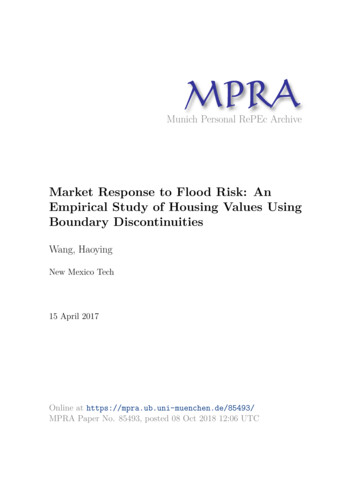
Juniata County. Flood events are observed in the region frequently. For instance,Juniata County had 6,374 acres flooded during Tropical Storm Agnes in 1972, and 57families were seriously affected by the disaster (Juniata County PlanningCommission, 2009). For Perry County, 29 of its 30 municipalities are flood prone.Table A1 and A2 in the appendix report a list of major flood events occurred in bothcounties within recent decades, mainly the most dangerous kind of floods – flashflood. When excessive amount of rainfall water fills up dry creeks or river beds (oftensmaller tributaries) connected to currently flowing creeks and rivers, it leads to flashfloods and can cause rapid rises of water in a short time. Flash floods often occurwith no forewarning. Juniata County and Perry County make it an ideal region tostudy flood risk impact on rural housing markets. The housing markets in bothcounties belong to the greater Harrisburg metropolitan area housing market. Asshown in Figure A2, the real unit housing price (converted to constant value usingHousing Price Index (HPI) of Harrisburg metropolitan area) on average increases overthe study period in both counties.Following the rationale of identification through boundary discontinuity, theresearcher matched 597 pairs of SFR properties (1194 observations) which had atleast one sale between 1980 and 2015 with both sale price and sale year recorded inJuniata County. For Perry County, similarly, 912 pairs of SFR properties are matchedamong properties which had at least one sale between 1980 and 2015. The matchingof properties is based on the nearest distance. The algorithm is described in detailsin Appendix B with a sample computer code. Figure 2 shows the location of all thematched SFR properties located in the 100-year floodplain (area inundated by 1percent annual chance of flooding) created by FEMA. The shaded area within thecounty boundary is the flood prone area (including all land use types) drawn basedon the 100-year floodplain.12
Figure 2: Flood prone area and location of observationsNote that this study only includes full-time SFR properties, since the valuation ofother types of residential properties (e.g. condos, multi-families, apartments,vacation homes, and mobile homes) may be structurally different. Among all the SFRproperty transactions, the researcher also excluded all of the love and affection sales(usually with a transaction price of 1). In the estimation sample, the researcherdropped all the sales with transaction price less than 500. Due to data limitation,the researcher only has access to the most recent sale record if multiple sales wererecorded on a property in the past. All the sale prices are converted to constantvalues in 2015 USD using the HPI of Harrisburg metropolitan area (both counties arein commuting distance to the city of Harrisburg) published by the Federal HousingFinance Agency. Table 1 summarizes all of the variables used to estimate theproposed empirical model in (9). Note that the assessed land value and the assessed13
building value do not add up to the housing price. This is normal because thedetermination of property assessment value follows a system (e.g. negotiationbetween homeowners and assessor’s office) quite different from the marketmechanism. However, the assessment value in general is highly correlated withstructural attributes (e.g. number of bedrooms and bathrooms) of the property. Thebasic model is estimated using ordinary least squares (OLS) with heteroskedasticityrobust standard errors. The main control variables in the model are housingcharacteristics which are supposed to capture any structural differences betweenpaired properties, as well as the distances to county seat and the city center ofHarrisburg.Table 1: Summary statistics of variablesCountyJuniataPerryIn 100 year flood zonemean (s. d.)mean (s. d.)JuniataPerryOutside 100 year flood zonemean (s. d.)mean (s. d.)Housing price (in 5.09)Unit housing price (in .74)Lot size (in ssed Land value (in ssessed Building value (in )Living space (in 1000 nce to Harrisburg (in Distance to county seat* (in 12597912VariableNumber of observations* The seat of Juniata County is in Mifflintown, Pennsylvania. The seat of Perry County is in NewBloomfield, Pennsylvania.From the summary statistics, one can see that properties in the 100-year flood zoneon average is cheaper than their counterparts outside the 100-year flood zone, interms of both overall price and unit price. One should also note that housing price inJuniata County is relatively lower than housing price in Perry County, which likelyreflects the fact that Perry County locates closer to the city of Harrisburg. Thissuggests that distance to the central business district should be controlled in theempirical model. To control for structural differences between matched propertiesas much as possible, the researcher uses housing price per sqft living space as14
dependent variable. Figure 3 plots the distribution of unit housing prices (note thatactual dependent variable in the empirical model takes logarithm transformation)inside and outside the flood zone, obtained through nonparametric kernel densityestimation. As shown in the graph, the distribution of unit housing prices outs
many flood-prone residential areas more flood resistant, though not necessarily flood proof. In general, it is unrealistic to expect people and businesses to move out of the flood zone. The additional costs of living in the flood zone, however, have to be accounted into the budget of housing consumption. Its impact on property values