WIXLIB

Getting Started: POWER Procedure F 7111You designate one of these components by a missing value in the input, in order to identify it as the resultparameter. The procedure calculates this result value over one or more scenarios of input values for all othercomponents. Power and sample size are the most common result values, but for some analyses the result canbe something else. For example, you can solve for the sample size of a single group for a two-sample t test.In addition to tabular results, PROC POWER produces graphs. You can produce the most common types ofplots easily with default settings and use a variety of options for more customized graphics. For example,you can control the choice of axis variables, axis ranges, number of plotted points, mapping of graphicalfeatures (such as color, line style, symbol and panel) to analysis parameters, and legend appearance.If ODS Graphics is enabled, then PROC POWER uses ODS Graphics to create graphs; otherwise, traditionalgraphs are produced.For more information about enabling and disabling ODS Graphics, see the section “Enabling and DisablingODS Graphics” on page 609 in Chapter 21, “Statistical Graphics Using ODS.”For specific information about the statistical graphics and options available with the POWER procedure, seethe PLOT statement and the section “ODS Graphics” on page 7280.The POWER procedure is one of several tools available in SAS/STAT software for power and sample sizeanalysis. PROC GLMPOWER supports more complex linear models. The Power and Sample Size applicationprovides a user interface and implements many of the analyses supported in the procedures. See Chapter 48,“The GLMPOWER Procedure,” and Chapter 90, “The Power and Sample Size Application,” for details.The following sections of this chapter describe how to use PROC POWER and discuss the underlyingstatistical methodology. The section “Getting Started: POWER Procedure” on page 7111 introduces PROCPOWER with simple examples of power computation for a one-sample t test and sample size determinationfor a two-sample t test. The section “Syntax: POWER Procedure” on page 7119 describes the syntax of theprocedure. The section “Details: POWER Procedure” on page 7213 summarizes the methods employed byPROC POWER and provides details on several special topics. The section “Examples: POWER Procedure”on page 7281 illustrates the use of the POWER procedure with several applications.For an overview of methodology and SAS tools for power and sample size analysis, see Chapter 18,“Introduction to Power and Sample Size Analysis.” For more discussion and examples, see O’Brien andCastelloe (2007); Castelloe (2000); Castelloe and O’Brien (2001); Muller and Benignus (1992); O’Brien andMuller (1993); Lenth (2001).Getting Started: POWER ProcedureComputing Power for a One-Sample t TestSuppose you want to improve the accuracy of a machine used to print logos on sports jerseys. The logoplacement has an inherently high variability, but the horizontal alignment of the machine can be adjusted. Theoperator agrees to pay for a costly adjustment if you can establish a nonzero mean horizontal displacement ineither direction with high confidence. You have 150 jerseys at your disposal to measure, and you want todetermine your chances of a significant result (power) by using a one-sample t test with a two-sided 0.05.

7112 F Chapter 89: The POWER ProcedureYou decide that 8 mm is the smallest displacement worth addressing. Hence, you will assume a true mean of8 in the power computation. Experience indicates that the standard deviation is about 40.Use the ONESAMPLEMEANS statement in the POWER procedure to compute the power. Indicate poweras the result parameter by specifying the POWER option with a missing value (.). Specify your conjecturesfor the mean and standard deviation by using the MEAN and STDDEV options and for the sample size byusing the NTOTAL option. The statements required to perform this analysis are as follows:proc power;onesamplemeansmean 8ntotal 150stddev 40power .;run;Default values for the TEST , DIST , ALPHA , NULLMEAN , and SIDES options specify a two-sided ttest for a mean of 0, assuming a normal distribution with a significance level of 0.05.Figure 89.1 shows the output.Figure 89.1 Sample Size Analysis for One-Sample t TestThe POWER ProcedureOne-Sample t Test for MeanFixed Scenario ElementsDistributionNormalMethodExactMean8Standard Deviation40Total Sample Size150Number of SidesNull Mean20Alpha0.05ComputedPowerPower0.682The power is about 0.68. In other words, there is about a 2/3 chance that the t test will produce a significantresult demonstrating the machine’s average off-center displacement. This probability depends on theassumptions for the mean and standard deviation.Now, suppose you want to account for some of your uncertainty in conjecturing the true mean and standarddeviation by evaluating the power for four scenarios, using reasonable low and high values, 5 and 10 for themean, and 30 and 50 for the standard deviation. Also, you might be able to measure more than 150 jerseys,and you would like to know under what circumstances you could get by with fewer. You want to plot powerfor sample sizes between 100 and 200 to visualize how sensitive the power is to changes in sample size forthese four scenarios of means and standard deviations. The following statements perform this analysis:

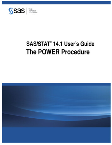
Computing Power for a One-Sample t Test F 7113ods graphics on;proc power;onesamplemeansmean 5 10ntotal 150stddev 30 50power .;plot x n min 100 max 200;run;ods graphics off;The new mean and standard deviation values are specified by using the MEAN and STDDEV options inthe ONESAMPLEMEANS statement. The PLOT statement with X N produces a plot with sample size onthe X axis. (The result parameter, in this case the power, is always plotted on the other axis.) The MIN andMAX options in the PLOT statement determine the sample size range. The ODS GRAPHICS ON statementenables ODS Graphics.Figure 89.2 shows the output, and Figure 89.3 shows the plot.Figure 89.2 Sample Size Analysis for One-Sample t Test with Input RangesThe POWER ProcedureOne-Sample t Test for MeanFixed Scenario ElementsDistributionNormalMethodExactTotal Sample Size150Number of Sides2Null Mean0Alpha0.05Computed PowerStdIndex Mean Dev Power15300.52725500.229310300.982410500.682

7114 F Chapter 89: The POWER ProcedureFigure 89.3 Plot of Power versus Sample Size for One-Sample t Test with Input RangesThe power ranges from about 0.23 to 0.98 for a sample size of 150 depending on the mean and standarddeviation. In Figure 89.3, the line style identifies the mean, and the plotting symbol identifies the standarddeviation. The locations of plotting symbols indicate computed powers; the curves are linear interpolationsof these points. The plot suggests sufficient power for a mean of 10 and standard deviation of 30 (for any ofthe sample sizes) but insufficient power for the other three scenarios.Determining Required Sample Size for a Two-Sample t TestIn this example you want to compare two physical therapy treatments designed to increase muscle flexibility.You need to determine the number of patients required to achieve a power of at least 0.9 to detect a groupmean difference in a two-sample t test. You will use 0.05 (two-tailed).The mean flexibility with the standard treatment (as measured on a scale of 1 to 20) is well known to be about13 and is thought to be between 14 and 15 with the new treatment. You conjecture three alternative scenariosfor the means:

Determining Required Sample Size for a Two-Sample t Test F 71151. 1 13, 2 142. 1 13, 2 14.53. 1 13, 2 15You conjecture two scenarios for the common group standard deviation:1. 1.22. 1.7You also want to try three weighting schemes:1. equal group sizes (balanced, or 1:1)2. twice as many patients with the new treatment (1:2)3. three times as many patients with the new treatment (1:3)This makes 3 2 3 18 scenarios in all.Use the TWOSAMPLEMEANS statement in the POWER procedure to determine the sample sizes requiredto give 90% power for each of these 18 scenarios. Indicate total sample size as the result parameter byspecifying the NTOTAL option with a missing value (.). Specify your conjectures for the means by usingthe GROUPMEANS option. Using the “matched” notation (discussed in the section “Specifying ValueLists in Analysis Statements” on page 7216), enclose the two group means for each scenario in parentheses.Use the STDDEV option to specify scenarios for the common standard deviation. Specify the weightingschemes by using the GROUPWEIGHTS option. You could again use the matched notation. But forillustrative purposes, specify the scenarios for each group weight separately by using the “crossed” notation,with scenarios for each group weight separated by a vertical bar ( ). The statements that perform the analysisare as follows:proc werntotalrun; (13 14) (13 14.5) (13 15)1.2 1.71 1 2 30.9.;Default values for the TEST , DIST , NULLDIFF , ALPHA , and SIDES options specify a two-sided ttest of group mean difference equal to 0, assuming a normal distribution with a significance level of 0.05.The results are shown in Figure 89.4.

7116 F Chapter 89: The POWER ProcedureFigure 89.4 Sample Size Analysis for Two-Sample t Test Using Group MeansThe POWER ProcedureTwo-Sample t Test for Mean DifferenceFixed ScenarioElementsDistributionMethodNormalExactGroup 1 Weight1Nominal Power0.9Number of Sides2Null DifferenceAlpha00.05Computed N TotalStdActualNIndex Mean1 Mean2 Dev Weight2 Power Total11314.0 1.210.9076421314.0 1.220.9087231314.0 1.230.9058441314.0 1.710.90112451314.0 1.720.90514161314.0 1.730.90016471314.5 1.210.9103081314.5 1.220.9063391314.5 1.230.91640101314.5 1.710.90056111314.5 1.720.90163121314.5 1.730.90876131315.0 1.210.91318141315.0 1.220.92721151315.0 1.230.92224161315.0 1.710.91434171315.0 1.720.92139181315.0 1.730.91044The interpretation is that in the best-case scenario (large mean difference of 2, small standard deviation of1.2, and balanced design), a sample size of N 18 (n1 D n2 D 9) patients is sufficient to achieve a power ofat least 0.9. In the worst-case scenario (small mean difference of 1, large standard deviation of 1.7, and a 1:3unbalanced design), a sample size of N 164 (n1 41, n2 123) patients is necessary. The Nominal Powerof 0.9 in the “Fixed Scenario Elements” table represents the input target power, and the Actual Power columnin the “Computed N Total” table is the power at the sample size (N Total) adjusted to achieve the specifiedsample weighting exactly.

Determining Required Sample Size for a Two-Sample t Test F 7117Note the following characteristics of the analysis, and ways you can modify them if you want: The total sample sizes are rounded up to multiples of the weight sums (2 for the 1:1 design, 3 forthe 1:2 design, and 4 for the 1:3 design) to ensure that each group size is an integer. To request rawfractional sample size solutions, use the NFRACTIONAL option. Only the group weight that varies (the one for group 2) is displayed as an output column, while theweight for group 1 appears in the “Fixed Scenario Elements” table. To display the group weightstogether in output columns, use the matched version of the value list rather than the crossed version. If you can specify only differences between group means (instead of their individual values), or if youwant to display the mean differences instead of the individual means, use the MEANDIFF optioninstead of the GROUPMEANS option.The following statements implement all of these modifications:proc weightspowerntotalrun; 1 to 2 by 0.51.2 1.7(1 1) (1 2) (1 3)0.9.;Figure 89.5 shows the new results.Figure 89.5 Sample Size Analysis for Two-Sample t Test Using Mean DifferencesThe POWER ProcedureTwo-Sample t Test for Mean DifferenceFixed ScenarioElementsDistributionMethodNominal PowerNumber of SidesNull DifferenceAlphaNormalExact0.9200.05

7118 F Chapter 89: The POWER ProcedureFigure 89.5 continuedComputed Ceiling N TotalMean StdIndex Diff Dev Weight1 Weight2Fractional ActualN Total PowerCeilingNTotal11.0 1.21162.5074290.9026321.0 1.21270.0657110.9047131.0 1.21382.6657720.9018341.0 1.711 123.4184820.90112451.0 1.712 138.5981590.90113961.0 1.713 163.8990940.90016471.5 1.21128.9619580.9002981.5 1.21232.3088670.9063391.5 1.21337.8933510.90138101.5 1.71155.9771560.90056111.5 1.71262.7173570.90163121.5 1.71373.9542910.90074132.0 1.21117.2985180.91318142.0 1.21219.1638360.91320152.0 1.21322.2829260.91023162.0 1.71132.4135120.90533172.0 1.71236.1955310.90737182.0 1.71342.5045350.90343Note that the Nominal Power of 0.9 applies to the raw computed sample size (Fractional N Total), and theActual Power column applies to the rounded sample size (Ceiling N Total). Some of the adjusted samplesizes in Figure 89.5 are lower than those in Figure 89.4 because underlying group sample sizes are allowed tobe fractional (for example, the first Ceiling N Total of 63 corresponding to equal group sizes of 31.5).

Syntax: POWER Procedure F 7119Syntax: POWER ProcedureThe following statements are available in the POWER procedure:PROC POWER options ;COXREG options ;LOGISTIC options ;MULTREG options ;ONECORR options ;ONESAMPLEFREQ options ;ONESAMPLEMEANS options ;ONEWAYANOVA options ;PAIREDFREQ options ;PAIREDMEANS options ;PLOT plot-options / graph-options ;TWOSAMPLEFREQ options ;TWOSAMPLEMEANS options ;TWOSAMPLESURVIVAL options ;TWOSAMPLEWILCOXON options ;The statements in the POWER procedure consist of the PROC POWER statement, a set of analysis statements (for requesting specific power and sample size analyses), and the PLOT statement (for producinggraphs). The PROC POWER statement and at least one of the analysis statements are required. The analysisstatements are COXREG, LOGISTIC, MULTREG, ONECORR, ONESAMPLEFREQ, ONESAMPLEMEANS, ONEWAYANOVA, PAIREDFREQ, PAIREDMEANS, TWOSAMPLEFREQ, TWOSAMPLEMEANS, TWOSAMPLESURVIVAL, and TWOSAMPLEWILCOXON.You can use multiple analysis statements and multiple PLOT statements. Each analysis statement produces aseparate sample size analysis. Each PLOT statement refers to the previous analysis statement and generates aseparate graph (or set of graphs).The name of an analysis statement describes the framework of the statistical analysis for which samplesize calculations are desired. You use options in the analysis statements to identify the result parameter tocompute, to specify the statistical test and computational options, and to provide one or more scenarios forthe values of relevant analysis parameters.Table 89.1 summarizes the basic functions of each statement in PROC POWER. The syntax of each statementin Table 89.1 is described in the following pages.Table 89.1 Statements in the POWER ProcedureStatementDescriptionPROC POWERInvokes the procedureCOXREGLOGISTICCox proportional hazards regressionLikelihood ratio chi-square test of a single predictor in logisticregression with binary responseTests of one or more coefficients in multiple linear regressionFisher’s z test and t test of (partial) correlationMULTREGONECORR

7120 F Chapter 89: The POWER ProcedureTable 89.1 continuedStatementDescriptionONESAMPLEFREQTests, confidence interval precision, and equivalence tests of asingle binomial proportionOne-sample t test, confidence interval precision, or equivalence testOne-way ANOVA including single-degree-of-freedom contrastsMcNemar’s test for paired proportionsPaired t test, confidence interval precision, or equivalence testDisplays plots for previous sample size EANSPLOTTWOSAMPLEFREQChi-square, likelihood ratio, and Fisher’s exact tests for twoindependent proportionsTWOSAMPLEMEANSTwo-sample t test, confidence interval precision, or equivalencetestTWOSAMPLESURVIVAL Log-rank, Gehan, and Tarone-Ware tests for comparing twosurvival curvesTWOSAMPLEWILCOXON Wilcoxon-Mann-Whitney (rank-sum) test for 2 independent groupsSee the section “Summary of Analyses” on page 7214 for a summary of the analyses available and the syntaxrequired for them.PROC POWER StatementPROC POWER options ;The PROC POWER statement invokes the POWER procedure. You can specify the following option.PLOTONLYspecifies that only graphical results from the PLOT statement should be produced.COXREG StatementCOXREG options ;The COXREG statement performs power and sample size analyses for the score test of a single scalarpredictor in Cox proportional hazards regression for survival data, possibly in the presence of one or morecovariates that might be correlated with the tested predictor.Summary of OptionsTable 89.2 summarizes the options available in the COXREG statement.

COXREG Statement F 7121Table 89.2 COXREG Statement OptionsOptionDescriptionDefine analysisTEST Specifies the statistical analysisSpecify analysis informationALPHA Specifies the significance levelSIDES Specifies the number of sides and the direction of the

Power and sample size analysis optimizes the resource usage and design of a study, improving chances of conclusive results with maximum efficiency. The POWER procedure performs prospective power and sample size analyses for a variety of goals, such as the following: determining the sample size required to get a significant result with .