Transcription
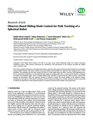
HindawiComplexityVolume 2018, Article ID 3129398, 15 pageshttps://doi.org/10.1155/2018/3129398Research ArticleObserver-Based Sliding Mode Control for Path Tracking of aSpherical RobotMajid Taheri Andani,1 Zahra Ramezani ,2 Saeed Moazami,1 Jinde Cao ,3,4Mohammad Mehdi Arefi ,5 and Hassan Zargarzadeh 11Phillip M. Drayer Electrical Engineering Department, Lamar University, Beaumont, TX, USAElectrical Engineering Department, Iran University of Science and Technology, Tehran, Iran3School of Mathematics, Southeast University, Nanjing 210096, China4Research Centre for Complex Systems and Network Sciences, Southeast University, Nanjing 210096, China5Department of Power and Control Engineering, School of Electrical and Computer Engineering, Shiraz University,Shiraz 71348-51154, Iran2Correspondence should be addressed to Hassan Zargarzadeh; hzargarzadeh@lamar.eduReceived 12 June 2018; Accepted 13 August 2018; Published 16 October 2018Academic Editor: Avimanyu SahooCopyright 2018 Majid Taheri Andani et al. This is an open access article distributed under the Creative CommonsAttribution License, which permits unrestricted use, distribution, and reproduction in any medium, provided the originalwork is properly cited.Due to their complicated dynamics and underactuated nature, spherical robots require advanced control methods to reveal all theirmanoeuvrability features. This paper considers the path tracking control problem of a spherical robot equipped with a 2-DOFpendulum. The pendulum has two input torques that allow it to take angles about the robot’s transverse and longitudinal axes.Due to mechanical technicalities, it is assumed that these angles are immeasurable. First, a neural network observer is designedto estimate the pendulum angles. Then a modified sliding mode controller is proposed for the robot’s tracking control in thepresence of uncertainties. Next, the Lyapunov theorem is utilized to analyse the overall stability of the proposed scheme,including the convergence of the observer estimation and the trajectory tracking errors. Finally, simulation results are providedto indicate the effectiveness of the proposed method in comparison with the other available control approaches.1. IntroductionSpherical robots are a class of rolling robots, which can beused in many applications: surveillance [1], environmentalmonitoring [2], exploration operations in unknown environments [3], rehabilitation [4], hobbies [5], and so on [6]. Dueto the ball-shaped shell, the enclosed components in a spherical robot are protected from collision and environmentalstates such as dust, humidity, and radiations. Spherical robotshave highly manoeuvrable dynamics that enjoy the advantage of never tipping over [7] and the minimum skiddingand resistance with the surface [8]. Nonetheless, the underactuated nature of these robots calls for advanced controlschemes to succeed with the path tracking problem [9, 10].Over the last few years, numerous studies have been conducted on modelling, point stabilization [11], and trackingcontrol of the spherical systems. The motion of the sphereunder rolling constraints is studied in [12]. In [13], two computationally path-planning algorithms are presented for therolling sphere. A first-order model for a spherical robot isderived in [14] from noninclined limitation and conservationof the angular momentum, as well as a path tracking methodwith minimum energy and time. In [15], a dynamic equationmodel is obtained for a spherical robot’s motion with amobile mass, which is placed inside the shell and it proposesits path planning on a surface with the presence of obstacles.Euler parameters are utilized in [16] to establish the kinematic equations for a spherical robot and represent thetrajectory planning problems. The dynamics model and control of a spherical robot with a driving wheel on the bottom ofthe sphere are investigated in [8] where the platform is notplain. The dynamics model of a spherical robot with a rolling
2mechanism consisting of a 2-DOF is studied in [17], and therotation matrices are derived to analyse the kinematics of thesystem. Then the Euler-Lagrange formalism is applied todevelop the decoupled dynamic modelling for the motionof the robot in transverse and longitudinal axes. Also, fuzzyand feedback linearization controllers are employed for thetrajectory tracking problem. In [18], utilizing the Lagrangemethod, the dynamics model and the motion control of apendulum-based spherical robot on an inclined plane wereinvestigated using a PID controller.In the literature, a variety of control schemes is introduced for the tracking control of spherical robots. By considering the spherical robot’s model, a backstepping feedbackcontroller for the kinematic equations is developed in [3].In [6], a real-time fuzzy guidance approach for the trajectorytracking of a 2-DOF pendulum spherical robot is introduced,with a focusing on simultaneous convergence of attitude andposition of the robot. The work in [19] proposes a neuralnetwork (NN) PID controller that has the advantages ofsimple forward and dynamic self-processing structure foran amphibious spherical robot. Modelling errors and uncertainties have motivated many researchers to utilize slidingmode control (SMC), as a kind of nonlinear robust controller[20, 21], for the spherical robot path tracking problem. Forexample, in [22], a 1-DOF spherical robot is modelled wherea SMC online learning method with fuzzy neural networkcontroller is used for velocity control of the robot. In [23], ahierarchical sliding mode is introduced to control the spherical robot in the presence of unwanted disturbances anduncertainties in real time.The aforementioned control approaches are designedwith the assumption that all the states of the system are measurable. Nonetheless, it is sometimes technically costly ormechanically impossible to measure all the states of the physical systems. To address this issue, linear and nonlinearobservers are introduced [24–26]. There have been numerous efforts conducted on estimating unknown parametersand immeasurable states in spherical robots. For instance,in [27], disturbance in an omnidirectional spherical robotis estimated, and then it is delivered to an observerbased generalized proportional integral (GPI) for cancelation of the disturbance. In [28], an extended observerbased adaptive hierarchical sliding mode for longitudinalmotion of the spherical robot is designed, in which theuncertain rolling resistance can be obtained without usingtraction sensors.In this paper, the trajectory tracking problem of a popularspherical robot is studied for a robot that uses a 2-DOF pendulum for driving the motion by moving the sphere’s masscentre, which creates gravitational torque [17]. While all therobot’s states need to be measurable for the controller design,the mechanical structure makes it a challenge to acquire thependulum angles using sensors. Even if sensors are installed,the acquired values may not be precise due to the noise andmeasurement delays. Besides, uncertainties and nonlineardynamics are intrinsic to spherical robots. To overcome theseproblems, in this paper, a sliding mode controller is introduced [29] that estimates the immeasurable states via aNN-based nonlinear observer [30].ComplexityNNs are widely utilized as adaptive observers to estimatethe system nonlinearities and the immeasurable states of thenonlinear systems [31]. Moreover, NNs are extensively usedin path tracking by mobile robots [27]. In [32], an adaptiveNN with a robust controller is applied to overcome the challenge of environmental border trajectory tracking of underactuated mobile robots with uncertain dynamics as well asthe presence of disturbances. In [33], the authors employan adaptive path tracking control with an interneural computing approach for a mobile robot to follow a moving target.This controller is a mathematical scheme that employs neuralpruning to the functions of rewards and punishment.Due to the complicated nonlinear dynamics, in thispaper, the spherical robot is modelled in a way that thedynamics are decoupled in two separated subsystems abouttransverse and longitudinal axes [17]. It is assumed that thependulum’s angles around these axes are immeasurable. Tomeasure the unknown states, a NN-based observer isdesigned that is adaptive against the robot’s nonlinearitiesand unknown parameters. Then an extended SMC is developed that uses the estimated states in the presence of themodel structural uncertainties. The SMC provides the torques for the spherical robot around transverse and longitudinal axes to track the desired trajectory. The proposedadaptive observer-based SMC not only rejects the uncertainties but can also estimate immeasurable states while therobot dynamics nonlinearities are assumed to be unknown.The Lyapunov theorem is utilized to guarantee that the overall closed-loop system is semiglobally uniformly ultimatelybounded (SGUUB). The performance of the proposed schemeis verified with application to the spherical robot for tracking a desired trajectory on the horizontal plane. To the bestknowledge of the authors, this is the first time that an adaptive observer-based SMC that estimates immeasurable stateshas been introduced to a nonlinear system in the presence ofuncertainties and unknown nonlinearities.The main contributions of this paper are as follows: (1)designing an observer to estimate immeasurable states, whichare the angles of the pendulum about transverse and longitudinal angles, (2) designing a radial basis function (RBF) neuralnetwork to approximate the uncertainties and nonlinearitiesof the robot model, and (3) designing a modified SMC thatguarantees the SGUUB of the overall closed-loop scheme inthe presence of the state estimation errors, uncertainties,and unknown nonlinearities.The rest of the paper is organized into six sections: themodel of the robot is introduced in the second section; inthe third section, kinematics and dynamics of the systemare introduced; in section four, an observer for the robot isdesigned; and section five presents an NN and SMC. Thesimulation results and comparison with relative approachesin the literature are discussed in section six, followed by theconclusions in the last section.2. Description of the Robot ModelIn this paper, a 2-DOF pendulum-driven spherical robot isstudied. The pendulum rolls the robot in two directions byshifting the sphere’s centre of gravity to different points.
Complexity3The schematic of this robot is shown in Figure 1. In thesphere, there are two aligned diagonal holes through whicha shaft is fixed to the sphere. A 2-DOF pendulum is hangedfrom the centre point of the shaft. As indicated in Figure 1,two motors are employed to provide torque, so the pendulum takes the required direction. Motor 1 rotates the pendulum about the sphere’s shaft that is considered as thetransverse shaft. Motor 2 rotates the shaft about the longitudinal axis about the horizon. Rotation of the pendulumabout the transverse axis moves the gravity centre towardsthe longitudinal axis, which causes the sphere to roll aboutthat axis. Rotating the pendulum about the longitudinal axismakes the sphere roll about the longitudinal axis. Therefore,by using two motors, the motion of the robot can be controlled over a flat surface.For deriving the dynamics model of the robot, it isassumed that two degrees of freedom do not have interactionon each other [17]; therefore, the equations of motion consistof two decoupled subsystems. With this assumption, themotions of a sphere on a flat surface (rolling without slipping) formulation of the kinematic and dynamic equationsare derived in [17].There exist three frames in Figure 2—oxyz represents thereference frames that is fixed to the ground, o1 x1 y1 z1 is themoving reference on the spherical centre that can translatewith respect to oxyz,, and o2 x2 y2 z2 is a moving reference tothe spherical centre which rotates with the sphere withrespect to o1 x1 y1 z 1 . The relative rotation angle of o2 x2 y2 z 2around o1 x1 is θ, and the relative rotation angle of o2 x2 y2 z 2around o1 y1 is ϕ. Figure 3 depicts the sphere’s turning motionabout its transvers axis. In Figures 2 and 3, θ, ϕ, and ψ are therotational angles of the robot around the o – x, o – y, and o – zaxes.3. Kinematics and Dynamics of theSpherical Robots3.1. Kinematics Equations. For deriving the kinematicsmodel, we use two rotations around the transverse and longitudinal axes. i, j, k T , i1 , j1 , k1 T , and i2 , j2 , k2 T denoteunit vectors which are attached to the oxyz C f ix , o1 x1 y1z 1 C 1 , and o2 x2 y2 z 2 C 2 coordinates, respectively. The firstrotation is written by the following transformation matrix.R1 Rot x, θ i1j1k100cos θ0 sin θ cos θi2 Rot x, θj2k2 Motor1Transverse axisMotor2Longitudinal axisPendulumFigure 1: Mechanical schematic of a 2-DOF pendulum-basedspherical robot. 휓z1z2 휃 훾1x2z 훾2x1 휌 훼yxIn this section, the kinematics and dynamics of the presentedspherical robot are expressed. Linear and turning motions ofthe robot are represented in Figures 2 and 3, respectively.1Vertical axis 휊Figure 2: Reference frames and kinematic schemes of rotationaround the transverse axis resulting in longitudinal motion. 휓 휙0sin θ , 훽100i20cos θsin θj20 sin θcos θk21Mp, IpFigure 3: Reference frames and kinematic schemes of rotationaround the longitudinal axis resulting in transverse motion of thesphere.
4ComplexityThe second transformation matrix for the second rotation is represented as follows:R2 Rot y, ϕ i1j1cos ϕ0 sin ϕ010sin ϕ0cos ϕcos ϕ 0i2 Rot y, ϕk1j2k2 centre of mass of the pendulum in two subsystems areas follows:V px V x ωpx r x ρθ h cos α θ α θ, h sin α θ α θjk,8 sin ϕi2010j2sin ϕ0cos ϕk2V pyAccording to Figure 2, the angular and linear velocities ofthe sphere are written as follows:ωs C f ix θi,V x ρθi,3jk3.2. Dynamics Equations. As mentioned in Section 2, forderiving the dynamics equations of the robot, it is considered that the degrees of freedom do not have interactionon the dynamics of each other, so the dynamic equationsconsist of two decoupled subsystems, in which the following assumptions are made:(1) Rotations about transverse and longitudinal axes donot have any interaction with each other(2) Around the vertical axis, there is no rotational motionV y ρϕj,where ρ is the radius of the sphere. The position of the centreof mass of the pendulum can be written as follows:r x C 2 h sin αj2 h cos αk2 ,4r y C 2 h sin βi2 h cos βk2 ,5in (4) and (5), α and β denote the angle of the pendulumabout transverse and longitudinal axes, respectively, and his the length of the shaft which connects the pendulum tothe center of the sphere. Using transformation matrices, theposition of the pendulum in the o1 x1 y1 z 1 coordinate is written as follows:rx C1 Rot x, θ rx C2 h sin α θ j1 h cos α θ k1 ,ry C1 Rot y, ϕ r y C 2 h sin β ϕ j1 h cos β ϕ k1 ,6where the position of the centre of mass of the pendulum infixed coordinate C f ix is equal to r x C 1 and r y C 1 . Theangular velocities of the pendulum in o2 x2 y2 z 2 and o1 x1 y1 z 1coordinates are written asωpx C 2 αi2 ,ωpx C1 ωs C 1 Rot x, θ ωpx C2 α θ i1 ,ωpy C 2 βj2 , r y ρφ h cos β φ β φ h sin β φ β φ2ωs C f ix ϕj, V y ωpy7ωpy C 1 ωs C1 Rot y, ϕ ωpy C2 β ϕ C 1 ,where the angular velocities in the fixed coordinates areppequal to ωx C1 and ωy C2 The linear velocities of theUsing the Lagrangian equations, dynamic equations ofthe systems can be derived. The Lagrangian formula for a system of particles can be defined byL T V,9where T is the total kinetic energy of the system and V is thepotential energy of the dynamic system. Since the kineticenergy of the system is equal to the kinetic energies of thewhole particles of the systems, the kinetic energy of the system is presented asT T s T p,10where T s and T p , are equal to the kinetic energy of the sphereand pendulum, respectively.11M V 2 I s ωs 2 ,2 s s21122T p M p V p I p ωp22Ts 11In (11), the moments of inertia of the sphere and pendulum areIs 2M ρ2 ,3 sIp 1hM h2 M p12 p2122,where M s and M p are masses; the weight of the sphere andpendulum, ωs , ωp , V s and V p , represents angular velocitiesof sphere and pendulum and linear velocities of them, respectively. As the centre of mass of the sphere remains in constantheight, the potential energy of the spherical robot depends on
Complexity5the pendulum’s mass and its vertical distance from the centreof the sphere.V M p gh1321 Mp2 h sin α θ α θ2X h cos α θ α θ 1I α θ2 p2112M Y I s ωy2 s22 M 41 M 42 0,M 43 M p ρh cos q4 q3 M p h2 I p ,M 44 M p h2 I p ,Z 11 M p gh sin q2 q1 M p ρh sin q2 q1 q222 M p ρh sin q2 q1 q21 2Mp ρh sin q2 q1 q1 q2 ,Z 21 M p gh sin q2 q1 , M p gh cos α θ ,Ly M 33 2M p ρh cos q3 q4 M p h2 M p ρ2 I p M s ρ2 I s ,M 34 M p ρh cos q4 q3 M p h2 I p ,Let us decouple (8) into (11) and decouple the Lagrangian equation into two parts based on rotation in the transverse axis Lx and vertical axis Ly .112Lx M s X I s ω x22M 23 M 24 M 31 M 32 0,1M2 p h sin β ϕ β ϕ22Y h cos β ϕ β ϕ1 Ip β ϕ2Z 31 M p gh sin q4 q3 M p ρh sin q4 q3 q24 M p ρh sin q4 q3 q23 2M p ρh sin q4 q3 q3 q4 ,2Z 41 M p gh sin q4 q3 M p gh cos β ϕ1714Euler’s equations for systems can be presented as follows:d Lx L x Qi ,dt qi qid Lydt q j15 Ly Qj, q jwhere qi expresses θ and α q1 θ, q2 α and representsgeneralized coordinates. Besides, Qi is considered as inputtorque in the transverse axis Q1,2 τx . Also, in the aboveequations, q j is equal to ϕ and β q3 ϕ, q4 β and theyare generalized coordinates. Q j represents input torque inthe longitudinal axis Q3,4 τy .Let us plug (14) into (15) and rearrange the derived equations in a united state space and write the equation of motionin the matrix form [17].M q t q t Z q t ,q t τ,16where τ τx , τx , τy , τy T ,M 11 2M p ρh cos q2 q1 M p h M p ρ I P M s ρ I s ,222The objective of this paper is to design a path trackingcontrol scheme for this robot, in the following sections: first,an observer will be designed to estimate the immeasurablestates; then an adaptive neural network observer-based sliding mode controller will be proposed.4. Observer DesignTo the best knowledge of the authors, in the works that havebeen done on the spherical robots, it is assumed that α andβ are available [17, 18, 23]. However, since all the parts ofthe spherical robot, installed in the shell, rotate about someaxis, measurement of α and β with sensors is costly orimpractical due to mechanical inaccessibility. To overcomethis problem, in this paper, an observer is designed to estimate the unavailable system states which are the degreesof freedom of the pendulum with respect to the transverseand longitudinal axes.Considering the dynamics of system (16), two outputs ofsystems are to be controlled via the two inputs. In this study,X and Y are the outputs and the torques are control inputsof the system. Let us transform the dynamic system into thefollowing form:q t M 1 Z q t , q tM 12 M p ρh cos q2 q1 M p h2 I p ,q1M 13 0,q2M 14 0,q3M 21 M p ρh cos q2 q1 M p h2 I p ,q4M 22 M p h2 I p , M 1 τ,τxZ 11 M 1Z 21Z 31Z 4118 M 1τxτy19τyIn order to design an observer, (19) can be rewritten inthe following state space form:
6Complexityx1 x2 ,represented in the following form:x2 f 2 x, u ,x Ax B h x Ω ,24x3 x4 ,x4 f 4 x, u ,20x5 x6 ,where x x, u, Ω T . Consider an observer represented asfollows:x̂ Âx k0 y ̂y ,x6 f 6 x, u ,x7 x8 ,x8 f 8 x, u ,where x ℜ8 1 are states of the system in which x1 θ,x3 α, x5 ϕ, x7 β, u τ ℜ4 1 , and f i x, u ℜ with i 2, 4, 6, 8 and f 2 x, u q1 , f 4 x, u q2 , f 6 x, u q3 , f 8x, u q4 .Moreover, (20) can be rewritten in the following form:26AT0 P PA0 Q,where F x, u f 2 x, u f 4 x, u f 6 x, u f 8 x, uCT x A0 x B h x Ω21y C T x,B where x̂ is the estimation of the vectors x and ̂y CT x̂.k0 ℜ8 4 is a vector which is called observer gain, and it istaken to make the characteristic polynomial of A0 A k0C T Hurwitz matrix. Defining the estimation error as x x x̂, we haveSince A0 is a Hurwitz matrix, there exists P ℜ8 8x Ax B F x, u ,A 0000 00010000 00000010 00000001 00Tand27and Q ℜ8 8 is an arbitrary positive definite matrix.Since C T x relies on available states, the strictly positivereal (SPR) Lyapunov design approach is used to guaranteethe stability of the closed-loop system [34]. Considering(26) as a linear system with h x Ω as its input, we defineH s C T sI A0 1 B. So, we have C T x H s h x Ω .The transfer function H s is known as a stable transfer function. In order to utilize the SPR-Lyapunov design approach,C T x H s h x Ω can be taken as,CT x H s L s L 1 s h x L 1 Ω ,22T28withLi s smi b1i smi 1 bmi mi 8 ,i 1, 2, , 4,L s diag L1 s , , L4 s,29L s is chosen, so that L 1 s is a proper stable transferfunction and H s L s is a proper SPR transfer function.Now, system (28) can be realized in state space as follows:,x A0 x Bc L 1 s h x Ω ,since θ, θ, ϕ, and ϕ are available and measurable states, theoutput matrix is considered to be CT .F x, u can be taken asF x, u F x, u Ω Ω h x Ω,23where h x ℜ4 1 and Ω ℜ4 1 are a neural network-basedaffinizing term that will be defined in (32). So, (21) can be30where BC is chosen such that PBC C.Moving on, h x needs to be approximated by utilizing aRBF neural network [35]. RBF is a neural network that isused in the practical applications for its simple structureand its capabilities of nonlinear function approximation[35, 36]. Afterwards, h x is used to develop an adaptive controller with its adaptation law to meet the control objectiveand guarantee boundedness of all signals in the closed-loopsystem. h x is approximated (z ΩNN ℜn is the input
Complexity7vector) by using RBF NN, as follows:ĥ x ψξ x ,T31where ψ ψ11 , ψ12 , , ψ1l is the weight vector of the neuralnetwork system function vector with l nodes and ψ1i ℜ4 l ,i 1, 2, , l. And ξ x ξ1 x , ξ2 x , , ξl x T is a basisfunction with Gaussian function ξi x exp x μi 2 /ηi 2 ,with centre μi μi1 , μi2 , , μil T and width η, and δ x, x̂ h x ĥ ̂x ψ is the neural network approximation error.The neural network controller is designed.Ω ψξ x̂33Assumption 1. δm L 1 s δ x, x̂ is bounded, i.e., δm δ.Consider the following Lyapunov function for systems (30)and (33):V1 1 T1x Px ψψT22γ34By calculating the time derivative of Lyapunov function andusing (27), we obtainV1 1 T T1 Tx A0 P PA0 x xT PBc L 1 s h x Ω ψψ2γ35In (35), h x ψξ x δ x, x̂ ψξ x̂ ψξ x̂ δ x, x̂ canbe approximated based on (31). Then by replacing neuralnetwork controller (32) in (35), we haveV1 1V 1 xT Qx xT PBc L 1 s ψξ x̂ ψξ x̂ ψξ x̂21 δ x, x̂ ψ γξ x̂ xT PBc L 1 sγ1 xT Qx xT PBc L 1 s δ x, x̂238So, based on Assumption (1), the above equation can be written in the following equation:32Hence, ψ ψ ψ where ψ is an estimate of ψ. Theadaptive law isψ γBTc PxL 1 s ξT x̂TNow, ψ ψ and then by using (33) in (37), we have1 T Tx A0 P PA0 x xT PBc L 1 s ψξ x̂ ψξ x̂21 T δ x, x̂ ψξ x̂ ψψγ1V 1 xT Qx xT PBc δ239In the above equation, based on Young’s inequality, we have xT PBc δ xT C δ 1x22 1 2δ,240and then we have11xV 1 xT Qx 222 1 21δ q0 x222 1 2δ,241where q0 λmin Q 1 and λmin Q is the minimum characteristic value of Q. So, the observer is provided; in the nextsection, the SMC is given to control the spherical robot.5. Sliding Mode ControlThe aim of this paper is designing a robust controller, so thespherical robot tracks a desired trajectory, where the torquesof the spherical robot about the transverse and longitudinalaxes are the system inputs. To that end, the controller forthe kinematics part of the robot will be designed. The kinematic models of the robot are written as follows.X ρθ,X ρθ,36Y ρφ,42Y ρφ,By replacing (27) in (36), we have:where X and Y are the position of the spherical robot. Bysubstituting θ and φ into (42) from (19), second derivativesof X, Y are calculated as follows:1V 1 xT Qx xT PBc L 1 s ψξ x̂ ψξ x̂ δ x, x̂21 T ψξ x̂ ψψγ37G D x J x U,43
8Complexity1X [m]0.50 0.5 10510151015XdX1Y [m]0.50 0.5 105Time (sec)YdYFigure 4: Robot trajectory around X and Y directions.withG X1,YJ x τxτy44,J 1,1 xJ 1,2 xJ 2,1 xJ 2,2 x J 1,1 x00J 2 ,2 xM 1 MA00MDM 1A00M 1D,45 1 1 0.50X [m]0.51Desired trajectoryTrajectoryInitial conditionFigure 5: Robot trajectory around the X – Y plane.measurement, the observer state estimation from the previous section will be used, i.e., the estimated states x̂ are usedinstead of the immeasurable states x .Taking the sliding surface,,where M A , M B ℜ . Therefore, in (43), J 1,2 x and J 2,1 xare zero. Since all the states are not available for2 20 0.5,where the first row of D x ℜ2 1 is derived from multiplying ρ and the first row of M 1 G and the second rowof D x is derived from multiplying ρ and the third rowof M 1 G. And, in J x ℜ2 2 , J 1,1 x and J 1,2 x arederived from multiplying ρ and the first row of M 1 ,and J 2,1 x and J 2,2 x are derived from multiplying ρ andthe third row of M 1 . One should note that from (17), thematrix M ℜ4 4 can be represented in a subblock-wise format as follows:M Y [m]U 0.5SxSy X XdY Yd λ10X Xd0λ2Y Yd e λe,46
Complexity90.10e(x) [m] 0.1 0.2 0.3 0.4 0.50510151015(a)1e(y) [m]0.80.60.40.20 0.205Time (sec)(b)Figure 6: Trajectory error around X and Y directions.where X d , Y d , and their derivatives are the desired position ofthe robot’s centre and its linear velocity. λ1 and λ2 are strictlypositive and constant values. The derivative of the slidingsurface is calculated asSt SxSy X XdY Yd λ10X Xd0λ2Y Yd47To reach trajectory tracking, S t should remain zero aslong as the robot is moving. So, the following equivalent control law ueq is taken:ueq JGd Gd ς 1,,48 kς 1 sgn S λ G Gdus inv J x̂S Sx,Sywhere γ is a constant value. One should note that J isinvertible due to the invertibility of M. As mentionedabove, trajectories should reach a sliding manifold in a limited bound and remain being bound in the presence of,50K100K2,where K 1 , K 2 are positive design parameters. Also, we takethe Lyapunov stability theorem for this system as follows:Yd112,1 1249where us is taken for robust stability of the spherical robotin facing uncertainties and unmodelled dynamics.k YdXdU ueq us , 1x̂ D x̂ Gd γς S ,Xduncertainty and unmodelled dynamics. Hence, the controllaw U is taken asV2 1 TS ςS251By considering the sliding surface in (46), the controlsignal isU J 1 x̂ D x̂ Gd γς 1 S kς 1 sgn S λ G Gd52
10Complexity2 휏x [N.m]1.50.10.50 0.5 10510151015(a)3 휏y [N.m]210 1 2 305Time (sec)(b)Figure 7: The input torques applied to the robot.The derivative of Lyapunov function with respect totime is1V 2 t ST ς G Gd λ G Gd0.5Y [m] ST ς D x̂ J x̂ U Gd λ G Gd053 0.5By replacing U in (53), we have 1V 2 t S ς D x̂ J x̂ JT 1 1x̂ D x̂ Gd γς S kς 1 sgn S λ G Gd ST γS k sgn S γ S 10.50X [m] Gd λ G Gd2 k S2 γ k S254 0.51Desired trajectoryTrajectoryInitial conditionFigure 8: Robot trajectory in the X – Y plane.Now, the design of the observer-based SMC is completeand the steps of the design can be summarized as the following steps: first, designing a NN-based observer whosestability is studied in (34) and developing a SMC for tracking control of the spherical robot using the Lyapunov function in (51) with the stability analysis in (53). Now, we areready to prove the overall stability of the proposed controller in the following theorem.V V1 V255By replacing (41) and (54) in the time derivative of V,it takes the following form:1V V 1 V 2 q0 x22 1 2δ γ k S2256By defining ζ γ k and by choosing k γ, we have1V q0 x22 1 2δ ζ S2257
Complexity111X[m]0.50 0.5 105XdX101510151Y[m]0.50 0.5 150Time (sec)YdY(a)6 휏x [N.m]420 2 4 605051015101510 휏y [N.m]50 5 10Time (sec)(b)Figure 9: (a) Robot trajectory tracking performance around the X and Y directions in the presence of measurement noise. (b) Input torquesapplied to the robot in the presence of the measurement noise.
12Complexitythat indicates V 0 as long as1.5q0x δ2,0.5Y [m]or2δ2ζS 59e 0.5 1.5 1.52δ,2ζλmin0 1Since S e diag λ1 , λ2 e,, (59) implies that [37]1158 1 0.5060where λmin min λ1 , λ2 . Now, from (57), (59), and (60)one can conclude that (x, ψ, e) are semi globally uniformly2q0 /δ and 1/λminultimately bounded with the bounds of0.51 1.5X [m]Feedback linearizationSMCObserver-based SMCInitial conditionDesired trajectoryFigure 10: Comparing the observer-based SMC performance withthe SMC and feedback linearization controllers in the X – Y plane.2δ /2ζ for x and e, respectively.The next section is dedicated to the numerical evaluationof the proposed controller and comparing it with othercontrollers in the literature.The positive definite matrix Q 10I 8 8 is chosenwhere I 8 8 is an identity matrix. Besides, A0 is computedas follows:6. Simulation Results6.1. Path Tracking. This section provides the simulationresults through MATLAB, to verify the efficiency of thedesigned trajectory tracking controller observer-based SMCrepresented. The parameters of the spherical robot areM s 3 (kg), M p 2 (kg), ρ 0 2 (m), l 0 075 (m), andg 9 81 (m/s2). Simulation is carried out with initial conditions as follows:Gd G t0 XdYdsin t X 0 Y 0,cos t61 13900 140 14000 2 200 2 200 140 14001 140 14000 2 200 2 200 140 14000 140 1390
Research Article Observer-Based Sliding Mode Control for Path Tracking of a Spherical Robot Majid Taheri Andani,1 Zahra Ramezani ,2 Saeed Moazami,1 Jinde Cao ,3,4 Mohammad Mehdi Arefi ,5 and Hassan Zargarzadeh 1 1Phillip M. Drayer Electrical Engineering Department, Lamar University, Beaumont, TX, USA 2Electrical Engineering Department, Iran University of Science and Technology, Tehran, Iran