Transcription
Counting SAT-based Weighted PlanningŞtefan AndreiLamar University,Computer Science Department,sandrei@my.lamar.edu Peggy DoerschukLamar University,Computer Science Department,pdoerschuk@my.lamar.eduMartin RinardMIT, Department of ElectricalEngineering and Computer Science,rinard@lcs.mit.eduAbhishek MadaanLamar University,Computer Science Department,amadaan@my.lamar.eduJuly 2, 2009AbstractAutomated planning is one of the most important problems in artificial intelligence. We present a new refinement of the classical planning algorithm thatformulates the planning problem as a satisfiability problem. Compared withprevious techniques, the solution of the planning problem is identified usingthe number of truth assignments of the corresponding propositional formulaand their actions’ utilities. Our approach eliminates backtracking and supports efficient planners that consider additional subformulas without the needto recompute solutions for previously provided subformulas. The experimentalresults show that our approach can help existing SAT-based state-of-the-artplanners to find the solution plan more efficiently.1IntroductionPlanning is one of the most studied problems in artificial intelligence. Automatedplanning has many potential applications, from assisting in the management of logistics to minimising the impact of faults in a given system, assisting robots to dovarious activities, and so on. A planning problem is solved by a planner, which This paper is an improved and unified presentation of conference papers [2] and [3]. It containsa new section (Section 5) and complete proofs for the theoretical results (e.g., Lemma 4.1, 4.2, andTheorem 4.1), new definitions and more comprehensive experimental results.1
takes as input a description of an initial state, a goal, and the possible actions thatcan be performed in a given world. The output of the planner is a sequence ofactions which, when executed in any world satisfying the initial state, will achievethe desired goal.A planning problem can be viewed as a reachability analysis problem. Given aset A of actions, a state s is reachable from some initial state s0 if there is a sequenceof actions in A that defines a path from s0 to s. Reachability analysis consists ofanalyzing which states can be reached from s0 in some number of steps and how toreach them. Reachability can be computed exactly through a reachability tree or areachability graph, but these data structures lead to an algorithm with exponentialcomplexity.This exponential complexity motivated the introduction of the planning graph [7],a data structure that provides an efficient way to estimate the set of propositionspossibly reachable from an initial state under some set of actions. Planning graphshave polynomial size and can be built in polynomial time. But because the planninggraph provides only an approximation of the reachability tree, algorithms that usethe planning graph may need to backtrack to find a solution [9], which again leadsto exponential time complexity in the worst case.Researchers have also developed algorithms that formulate the planning problemas a propositional satisfiability problem [11–13], then use an off-the-shelf satisfiabilitysolver to obtain a solution. Recent improvements in the performance of generalpurpose algorithms for propositional satisfiability provide the ability to scale up torelatively large planning problems [10, 14].There exist already efforts to improve and extend the planning graph approach.For example, temporal planning [6] extends classical planning by considering timean important factor to determine the solution of the planning problem. Moreover,the temporal planning problem can often benefit from the concurrent execution ofactions. Another useful extension is probabilistic planning [15], where the uncertainty is in the actions’ effects. That is, each action has more than one outcomehaving a certain probability. Depending on the current state and action, the nextstate is decided according to its probability.Our method is a new extension of the classical planning graph approach byadding utilities to the actions [3]. This makes our approach different than both thetemporal and the probabilistic planning approaches. For example, in our approachthere is only one outcome associated with an action (not more than one as in theprobabilistic planning). In contrast, our weighted planning associates utilities toactions for making possible a global comparison between them. This paper continuesthe classical planning graph approach based on counting satisfiability illustratedin [2].2
1.1Planning graphBriefly, a planning graph is a directed layered graph, where arcs are permitted onlyfrom one layer (also called level) to the next. Nodes in level 0 of the graph correspondto the set P0 of propositions (or facts, literals) denoting the initial state of a planningproblem. To search for a solution, the planning graph is iteratively expanded forthe next level. Any level i from 1 to k contains two layers: an action level Ai (set ofactions whose preconditions are nodes in Pi 1 ) and a proposition level Pi (union ofPi 1 and effects of Ai ). The planning graph has arcs from the proposition level tothe action level, and from the action level to the next proposition level, that is, theaction’s effects. From this perspective, a planning graph can be viewed as a bipartitegraph, compared with the reachability graph. We can say that the planning graph(that has a polynomial size) is just an approximation of the reachability graph (thatmay have an exponential size in the worst case).A plan Π with k levels is a sequence of sets of actions Π hπ1 , π2 , ., πk i , withπi Ai , i 1, 2, ., k. Actions from πi can be executed in parallel, in the sensethat their execution order is immaterial. Two actions a1 and a2 are dependent if:(i) a1 deletes a precondition of a2 or(ii) a1 deletes an effect of a2 or(iii) a2 deletes a precondition of a1 or(iv) a2 deletes an effect of a1 .Two actions a1 and a2 from level Ai are mutex (i.e., mutually exclusive) if either:(i) a1 and a2 are dependent or(ii) a precondition of a1 is mutex with a precondition of a2 .Two propositions p1 and p2 from Pi are mutex if every action in Ai that has p1as an effect is mutex with every action that produces p2 , and there is no action inAi that produces both p1 and p2 [9]. In fact, when constructing the planning graph,propositions and actions monotonically increase from one level to the next, whilemutex pairs monotonically decrease. This implies that it is likely for the solutionto have more parallel actions close to the last generated level rather than the firstlevels.1.2Existing plannersGraphplan was the first planner to solve planning problems using planning graphanalysis [7]. Graphplan broke previous records in terms of raw planning speed, and3
has become a popular planning framework. The most important contribution ofGraphPlan was designing an efficient algorithm that is using the planning graph.Basically, the brief pseudocode of Graphplan [9] is:for (k 0, 1, 2, .) {expand the planning graph up to level k;check whether the planning graph satisfies a necessarycondition for plan existence for goal g;if it does, then call SolExtract(g, k);}where SolExtract(g, k) is given by:{if k 0 return the solution;for (each proposition p in g)nondeterministically choose an action from level k 1to achieve pif (any pair of chosen actions is mutex) do backtrack;g 0 {preconditions of chosen actions};recursive call SolExtract(g 0 , k 1);}Note that if there is a failure at level k during solution extraction, the algorithm willbacktrack over the other subsets of Ak 1 . If level 0 is successfully reached, then thecorresponding sequence is a solution plan. The set of solution plans is the cartesianproduct of all the disjunctions for the goal of level k (details in Sections 3 and 4).SATPLAN [10, 14] uses a similar approach, but there are some differences aswell (SATPLAN takes as input a set of axiom schemas, while Graphplan takes asinput a set of STRIPS-like operators). STRIPS is a formalism for describing actionsin a planning problem, and represents a shorthand for STanford Research InstituteProblem Solver. A STRIPS action is formed by a precondition and an effect. Anaction’s precondition is a set of properties or facts that must hold for the action tobe executed, and its effect is the changes of state (i.e., a new set of facts) that suchexecution will produce.1.3Our contributionThe contributions of this paper are: we provide a new automatic way to eliminate backtracking while searching fora plan. This is based on using the counting SAT problem and associating utilitiesfor the set of actions;4
our approach considers two more pieces of information that help to deterministically choose the proper actions for the solution plan: the increment and theaction’s utility; the technique is applied incrementally, namely we consider the satisfiabilityof the new added subformulas without repeating the satisfiability of the formersubformulas; the experimental results show that our planner can improve the efficieny ofstate-of-the-art SAT-based planners.The next section shows a general technique to automatically decide whether it isnecessary to extend the planning graph or to provide a solution plan. The idea is toconstruct a propositional formula F such that there exists a plan if and only if F issatisfiable.2A SAT encoding of the planning problemThe architecture of a typical planner has a compiler (which guesses a plan length,and generates a propositional formula), a simplifier (which shrinks the propositionalformula by applying techniques such as unit clause propagation and pure literalelimination), a solver (which finds a truth assignment of the propositional formula),and a decoder (which gives a solution plan).Let LP be the propositional logic over the finite set of atomic formulæ (propositional variables) V {X1 , ., Xn }. A literal L is an atomic formula A (positiveliteral) or its negation A (negative literal), and denote V(L) V(L) A. If V {X1 , ., Xn } is a set of atomic formulæ, then V denotes the set { X1 , ., Xn }. Theoperator V can be extended from a single literal to a set of literals as V : V V V , such that given a set S V V , then x V(S) if and only if x S V orx S V . In other words, V(S) enumerates all the atomic formulæ from S. Forexample, V({A, B, C, A}) {A, B, C}.Any function S : V {0, 1} is an assignment (or, model), and it can be uniquelyextended in LP to F . Any propositional formula F LP can be translated into theconjunctive normal form (CNF): F (L1,1 . L1,n1 ) . (Ll,1 . Ll,nl ), whereLi,j are literals and l 1. We shall use the set representation {{L1,1 , ., L1,n1 }, .,{Ll,1 , ., Ll,nl }} to denote F . This set representation makes the notations easier tobe defined than the traditional representation. However, not all occurrences of the‘comma’ operator above have the same meaning. Note that the internal ‘comma’operator corresponds to the ‘ ’ boolean operation, while the ‘comma’ operator external to the set of literals corresponds to the ‘ ’ boolean operation. Any finitedisjunction of literals is a clause and a formula in CNF is called a clausal formula.A formula F is called satisfiable iff there exists a structure S for which S(F ) 1.5
A formula F is called unsatisfiable (or contradiction) iff F is not satisfiable. Wedenote by the empty clause (i.e., the one without any literal). A unit clause hasonly one literal.There are many ways of generating the CNF formula for a planning problem [9].One way is to consider the following five types of formulas:1) the initial state is encoded as the conjunctive of facts that hold and the negation of those that do not hold;2) the set of goal states is encoded as the conjunction of facts that must hold inthe last state;3) the A P, E axioms: given an applicable action, its preconditions must holdat that step, and its effects will hold at the next step;4) the explanatory frame axioms: if a fact changes, then one of the actions thathave that fact in its effects has been executed;5) the complete exclusion axioms: only one action occurs at each step.These five sets of formulas encode the planning problem P having a goal with nactions to propositional satisfiability [11]; that is, the CNF formula is satisfiable iffthere exists a solution plan of length n to P. Since only one action occurs at eachlevel, this is also called linear SAT-encoding.There exist variations of the above encoding, with the possibility of doing morethan one action at each level, for example by considering classical frame axiomswhich state what facts are left unchanged by a given action [16]. In this case,exclusion axioms are unnecessary since the classical frame axioms combined withA P, E axioms ensure that any two actions occurring at time t lead to identicalworld-state at time t 1.Another variation refers to exclusion. Instead of complete exclusion axioms,only the conflict exclusion axioms [8] may be added (two actions conflict if one’sprecondition is inconsistent with the other’s effect).Another possible SAT encoding was shown in [13], where the planning graph canbe automatically converted into a CNF formula by considering: the initial state and goal encodings, the encoding of ‘mutex of conflicting actions’, the encoding of ’actions imply their preconditions’, the encoding of ‘each fact implies the disjunction of all corresponding operators(actions, facts) from the previous levels’.6
Among all the existing SAT-encodings, it seems this latter one is the most efficient because of the CNF formula size. As mentioned in [13], this encoding ismore efficient than Graphplan-based encodings when considering larger benchmarkinstances. However, this SAT-encoding is not complete, in the sense that not everysolution of the SAT formula corresponds to a solution of the planning problem. Because of the lack of axioms of kind ‘actions imply their effects’, the SAT solutionsmay contain spurious actions. In fact, this matter was solved in [11], where theextraction function can simply delete actions from the solution whose effects do nothold. We use in our approach the SAT encoding from [13].3Our ApproachThis paper presents a new planning algorithm. Like the standard SAT-based algorithms, our technique is based on reducing the planning graph to a SAT problemand solving it as an incremental counting SAT problem.A counting problem P determines how many solutions exist, not just an answer“Yes/No” like a decision problem. The problem of counting the number of truthassignments (denoted by #SAT) was proved to be #P-complete [18]. The #Pcomplete problems are at least as hard as N P-complete problems. In fact, the class#P includes N P, and, in turn, is included in PSPACE.For a finite set A, A denotes the number of elements of A. Z, N and N denote the set of integers, positive integers, and the set of strict positive integers,respectively.Notation 3.1 Let C1 , ., Cs be clauses over V (s 1). We denote:a) mV (C1 , ., Cs ) {A A V V(C1 . Cs )} ;b) difV (C1 , ., Cs ) 0 if ( i, j {1, ., s}, i 6 j, such that L Ci and L Cj )or ( i {1, ., s}, such that Ci ); otherwise, difV (C1 , ., Cs ) 2mV (C1 ,.,Cs ) ;c) the determinant of the set of clauses {C1 , ., Cs } is detV (C1 , ., Cs ) 2 V sPP( 1)j 1 ·difV (Ci1 , ., Cij );j 11 i1 . ij sIn other words, the above notation says that mV (C1 , ., Cs ) denotes the numberof atomic formulae from V which do not occur in C1 . Cs . The positive integernumber difV (C1 , ., Cs ) is 0 iff there is a literal in one of the argument’s clause andits opposite in another clause or one of the clauses is the empty one. The integerdetV (C1 , ., Cs ) is a sign-alternated sum of difV (). If F {C1 , ., Cs }, we maydenote mV (C1 , ., Cs ) as mV (F ), difV (C1 , ., Cs ) as difV (F ) and detV (C1 , ., Cs ) asdetV (F ). In fact, the determinant of a clausal formula coincides with the number oftruth assignments of that formula. Given F LP over V , there exist detV (F ) truth7
assignments for F. Obviously, knowing detV (F ), the SAT problem can be solved,too. That is, F is satisfiable iff detV (F ) 6 0.For example, let us consider F {C1 , C2 , C3 }, where V {p, q, r} and C1 {p, q}, C2 {q, r}, C3 {p, r}. Then mV (C1 ) 3 2 1, mV (C1 , C2 ) 3 3 0,and so on. Thus, difV (C1 ) 2, difV (C1 , C2 ) 0, and so on. Therefore, detV (F ) 23 (21 21 21 ) 20 3. It follows that F is satisfiable and has detV (F ) 3(distinct) truth assignments.Incremental computation: Since detV (F ) may contain an exponential numberof difV ()’s depending on the number of clauses of F , whenever a new clause C isadded, it is better to compute only the difV ()’s which contain C and not the wholedifV ()’s corresponding to F {C}. Next, the increment of a given clausal formulaF with an arbitrary clause C is defined.Notation 3.2 If F {C1 , ., Cl } is an arbitrary clausal formula over V and C islPPan arbitrary clause over V , then incV (C, F ) ( 1)s 1 ·difV (C, Ci1 ,s 01 i1 . is l., Cis ) is called the increment of F with clause C.The increment is a negative integer representing the number of truth assignmentswhich have to be added or subtracted from the previous value of the determinant.In the following, the main result of this section is presented. It allows the computation of the determinant of a new clausal formula using the already computeddeterminant of the old clausal formula. Moreover, the incremental computationof the determinant of a formula containing new clauses is optimal. That is, nonew difV ()’s expressions are computed in the new incremental expression, that isincV (C, F ), except the ones which would have been created in the non-incrementalapproach.Theorem 3.1 [1] Let F {C1 , ., Cl } be a clausal formula over V and letF 0 {Cl 1 , ., Cl k }, k 1, be a clausal formula over V . Then detV (F F 0 ) detV (F ) incV (Cl 1 , F ) incV (Cl 2 , F {Cl 1 }) . incV (Cl k , F {Cl 1 } . {Cl k 1 }).Considering notations from Theorem 3.1, we denote incV (F 0 , F ) incV (Cl 1 , F ) incV (Cl 2 , F {Cl 1 }) . incV (Cl k , F {Cl 1 } . {Cl k 1 }). The nextcorollary points out some situations when the computation of the determinant andthe increment can be sped up.Corollary 3.1 [1] Let F {C1 , ., Cl } be a clausal formula over V . Then:a) if A is a new atomic variable, A / V , then detV {A} ({A}, F ) detV {A} ({A}, F ) detV (F ) and incV {A} ({A}, F ) incV {A} ({A}, F ) detV (F );8
b) if V 0 {X1 , ., Xm } is a set of atomic variables, m N , X1 , ., Xm / V,then detV V 0 (F ) 2m · detV (F ) and incV V 0 (C, F ) 2m · incV (C, F ).We define a utility function as u : A R, where A is the set of actions andR is the set of real numbers. Given an action Ai , the equality u(Ai ) x meansthe weight of Ai is x. The motivation of considering such a weight function is formaking a distinction between the actions, such as safety or efficieny or other reasons.For example, the action A1 “take the lift” is more efficient (or convenient) thanthe action A2 “go by stairs”, especially when there are many floors to walk.However, in case of a fire, action A2 is safer than action A1 . If we take the efficiencyas a utility measure, then a possible assignment for the utility function could beu(A1 ) 3 and u(A2 ) 1. If we take instead the safety as a utility measure, then aproper assignment for the utility could be u(A1 ) 1 and u(A2 ) 2. Our approachdoes not have a predefined algorithm for assigning the utility values to the actions.The responsibility to assign proper values for the utility function belongs to theplanning problem designer. As a general rule, different actions have different utilityvalues.Let us denote by L the set of levels, that is, {1, ., k} is the set of all levels bylevel k. Given a set of actions A {A1 , ., An } from level i L, we extend theutility function from an action to a set of actions by defining u : A L R, whereu(A, i) u(A1 ) . u(An ), where A A and i L. This can be generalizedin turn to a solution plan Π hπ1 , π2 , ., πk i , by defining u(Π) 1 · u(π1 ) . k · u(πk ), where πi Ai is the set of actions from level i, i 1, 2, ., k. Whenhaving to choose between many plans of different utilities, our method will alwayschoose the plan with maximum utility. In fact, the actions’ utilities are very usefulwhen the planner has to determine the solution plan (details in Section 4).3.1Our running exampleTo illustrate our technique, we choose as running example the “dinner-date” examplefrom [19]. Its specification can be made using STRIPS-like domains:Initial state: (and (garbage) (cleanHands) (quiet))Goal: (and (dinner) (present) (not (garbage)))Actions:cook: precondition (cleanHands): effect (dinner)wrap: precondition (quiet): effect (present)carry: precondition: effect (and (not garbage)) (not (cleanHands)))9
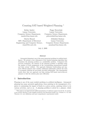
dolly: precondition: effect (and (not garbage)) (not (quiet)))The designer of this problem decides to choose the following utilities for theactions: u(cook) 5, u(wrap) 6, u(carry) 7, and u(dolly) 3. It is recommended that the utilities be different for different actions. The utility for dollyis the smallest as the husband wants to achieve all his goals before his wife, Dolly,wakes up.In this example, it is supposed that someone has initially cleanHands, while thehouse has garbage and is quiet. There are four possible actions: cook (requirescleanHands and achieves dinner), wrap (requires quiet and produces present),carry (has no precondition, but it has two effects: removes garbage, and negatescleanHands), and dolly (with no precondition, but she may remove the garbageand negates quiet). The planning graph up to level 1 is given in Figure 1 [19]. Actionnames are surrounded by boxes and horizontal double lines denote maintainanceactions. Thin, curved lines between actions and propositions at a single level denotemutex relations.garbgarbcarry garbdollycleanHcleanHcookquiet cleanHquietwrap quietdinnerpresent dinner dinner present presentP0A1P1Figure 1. The dinner-date planning graph (levels 0, 1)Obviously, we have two pairs of mutex actions: carry with cook, and dollywith wrap. Moreover, there exist two mutex pairs of propositions at level 1, namely cleanH (shortcut for cleanHands) with dinner, and quiet with present.It is easy to check that all propositions from the goal are possible at level 1, sincethey are not mutex with each other. Thus, there is a chance that a plan exists.10
Graphplan will consider two sets of actions: {carry, cook, wrap} and {dolly, cook,wrap}. Unfortunately, none of these sets of actions is a solution since carry is mutexwith cook while dolly is mutex with wrap. Because the solution extraction fails,Graphplan will extend planning graph with one more level.For efficiency reasons, we consider the SAT encoding from [13] and illustratehow it works for the dinner-date example [19]. Even if this SAT encoding is anincomplete one, there exist different ways to find the proper solution (details inSection 3). The fact that the planning graph having one level cannot lead to asolution can be automatically done by checking the satisfiability of a CNF formulawhich encodes the given problem. Let us denote by V1 {X1 , X2 , ., X14 } the set ofpropositional variables which corresponds to garbage, cleanHands, quiet, dinner,present (from level 0), carry, dolly, cook, wrap, garbage, cleanHands, quiet,dinner, present (from level 1), respectively. The initial state corresponds to theformula: { {X1 }, {X2 }, {X3 }, {X4 }, {X5 } }. The goal for the first level is: { {X10 },{X13 }, {X14 } }. For example, by considering the ‘actions imply their preconditions’axioms, we get the clauses {X2 , X8 }, {X3 , X9 }, by considering the mutex betweenactions axioms we get {X6 , X8 }, {X7 , X9 }, and by considering ‘each fact implies thedisjunction of all operators’ axioms we get {X6 , X7 , X10 }, {X8 , X13 }, and {X9 , X14 }.garb garbgarbcarry garbdollycleanH cleanHquiet quietcleanHcookwrap cleanHquiet quietdinnerdinnerpresentpresent dinner dinner present presentP1A2P2Figure 2. The dinner-date planning graph (level 2)We denote by F1 the CNF formula containing all the previous clauses. Since F1is unsatisfiable, there is no solution for the planning graph having only one level.Figure 2 shows the planning graph extended with one more level of actions and11
facts. In fact, a more efficient way to find the smallest k such that the planninggraph has at least a solution is to use the binary search method [13]. The binarysearch method applied to the planning problem has two steps:1. find a k such that the planning graph has a solution plan by generating aplanning graph with twice as many levels as the previous one (e.g., 1, 2, 4, 8,16, .);2. apply a ‘divide and conquer’ method by investigating the planning graph having the mean of the last two levels (that is, (k 2k)/2), etc.For example, if the first planning graph length that has solutions is 5 , the searchcan proceed for planning graphs of length 2, 4 (no solution plan found), 8 (solutionplan found), 6 (solution plan found) and finally 5.Let us denote by X15 , X16 , ., X23 the propositional variables which correspondsto carry, dolly, cook, wrap, garbage, cleanHands, quiet, dinner, present, allfrom level 2. The new set of variables is now V2 V1 { X15 , X16 , ., X23 }. Letus denote by F2 the CNF formula which encodes the planning graph up to level 2.Obviously, F2 contains F1 , except the goal clauses, and the following new clauses {{X19 }, {X22 }, {X23 } } (the goal for the second level), {X11 , X17 }, {X12 , X18 } (the‘actions imply their preconditions’ axioms), {X15 , X17 }, {X16 , X18 } (the mutex between actions axioms), {X10 , X15 , X16 , X19 }, {X13 , X17 , X22 }, and {X14 , X18 , X23 }(‘each fact implies the disjunction of all operators’ axioms)Since the old goal has been removed, we insert into F2 the unit clauses whichcorresponds to the new goal: {X19 }, {X22 }, {X23 }. This time F2 is satisfiable, sowe have to look for solutions by considering all the 12 possible disjunctions for thegoal of level 2, namely {carry2 , dolly2 , garb1 } {cook2 , dinner1 } {wrap2 ,present1 }. Eventually, by running the procedure solExtract(), a solution will befound. Note that the solution extraction procedure may need to do backtracking inorder to get the desired solution.Next section shows a different alternative by proposing a deterministic approachfor solving the planning problem using counting satisfiability and utilities associatedwith the actions, without needing to do backtracking.4Solution extractionThe solution extraction for our approach is similar to the classical solution extractionprocedure that needs backtracking (Section 1).In the following, we shall describe our approach for the dinner-date example.By simply computing the determinant as shown in the previous section, we get12
detV1 (F1 ) 0, and detV2 (F2 ) 172. The above and below values for the determinant and increment have been obtained by simply running our Java programminglanguage implementation that calculates the determinant. We immediately deducethat F1 is unsatisfiable and F2 is satisfiable. It implies there are no solutions at level1 and there might be some solutions at level 2. To check that, one way is to verifywhich of the 12 candidate solutions are solutions of the planning problem, i.e., theelements of the cartesian product {carry2 , dolly2 , garb1 } {cook2 , dinner1 } {wrap2 , present1 }. Since each of these cases refer to addition of exactly three unitclauses to F2 , the computation time of the corresponding determinants/incrementscan be done efficiently by applying Theorem 3.1. These are:(1)(1)(1) F2 {{X15 }, {X17 }, {X18 }} F2 , incV2 (F2 ) 172, so detV2 (F2 ) 0;(2)(2)(2) F2 {{X15 }, {X17 }, {X14 }} F2 , incV2 (F2 ) 172, so detV2 (F2 ) 0;(3)(3)(3) F2 {{X15 }, {X13 }, {X18 }} F2 , incV2 (F2 ) 132, so detV2 (F2 ) 40;(4)(4)(4) F2 {{X15 }, {X13 }, {X14 }} F2 , incV2 (F2 ) 132, so detV2 (F2 ) 40;(5)(5)(5) F2 {{X16 }, {X17 }, {X18 }} F2 , incV2 (F2 ) 172, so detV2 (F2 ) 0;(6)(6)(6) F2 {{X16 }, {X17 }, {X14 }} F2 , incV2 (F2 ) 132, so detV2 (F2 ) 40;(7)(7)(7) F2 {{X16 }, {X13 }, {X18 }} F2 , incV2 (F2 ) 172, so detV2 (F2 ) 0;(8)(8)(8) F2 {{X16 }, {X13 }, {X14 }} F2 , incV2 (F2 ) 132, so detV2 (F2 ) 40;(9)(9)(9) F2 {{X10 }, {X17 }, {X18 }} F2 , incV2 (F2 ) 144, so detV2 (F2 ) 28;(10)(10)(10) F2 {{X10 }, {X17 }, {X14 }} F2 , incV2 (F2 ) 152, so detV2 (F2 ) 20;(11)(11)(11) F2 {{X10 }, {X13 }, {X18 }} F2 , incV2 (F2 ) 152, so detV2 (F2 ) 20;(12)(12)(12) F2 {{X10 }, {X13 }, {X14 }} F2 , incV2 (F2 ) 172, so detV2 (F2 ) 0;(1)(2)(5)(7)(12)This SAT encoding ensures that F2 , F2 , F2 , F2 and F2do not correspond to solutions of the planning problem (because they are unsatisfiable formulas).(9)(10)(11)However, the formulas F2 , F2 and F2 correspond to satisfiable SAT formulas,but they do not lead to solutions of the planning problem. Since a classical SATsolver can only answer with ‘Yes/No’ regarding the satisfiability of a given CNF(9)(10)(11)formula, it is impossible to detect using a SAT solver that F2 , F2and F2cannot lead to solutions of the planning problem.To the best of our knowledge, there are two traditional ways to eliminate theincorrect (spurious) solutions: consider a richer SAT encoding, by including the A E axioms. However,this approach may lead to large SAT formulas; consider the above SAT encoding, but when the planning graph is created,special d
MIT, Department of Electrical Engineering and Computer Science, rinard@lcs.mit.edu Abhishek Madaan Lamar University, Computer Science Department, amadaan@my.lamar.edu July 2, 2009 Abstract Automated planning is one of the most important problems in artiflcial intel-ligence. We present a new reflnement of the classical planning algorithm that