WIXLIB

6wrong. Suffice it to say that clinical correlations are fundamental to the concept ofvalidity and are dependent on our knowledge of basic neuroanatomy andneurophysiology. These concepts are also dependent on our methods of measurementand the confidence one has in the mathematical simulations when applied in thelaboratory or clinical context. Today there are a wide number of fully testedmathematical and digital signal processing methods that can be rapidly evaluated usingcalibrated signals and a high speed computer to determine the mathematical validity ofany method and I will not spend a lot of time on this topic except for a brief mention of afew methods that are not valid when applied to coherence and phase measures because oftechnical limitations, for example, the use of an average reference or the Laplaciansurface transform and Independent Components Analysis (ICA) and the calculation ofcoherence and phase. It will be shown in a later section that the average reference andthe Laplacian distort the natural physiological phase relationships in the EEG and anysubsequent analyses of phase and coherence are invalidated when these remontaging orreconstruction methods are used (Rappelsberger, 1989; Nunez, 1981). The averagereference and Laplacian and ICA methods are valid for absolute power measures buthave limitations for phase measures which is a good example of why validity is definedas the extent to which a measuring instrument measures what it is intended to measure.Leaving the mathematical and simulation methods aside for the moment, the mostcritical factor in determining the clinical validity of qEEG is knowledge about theneuroanatomy and neurophysiology and functional brain systems because without thisknowledge then it is not possible to even know if a given measurement is clinically validin the first place. For example, neurological evaluation of space occupying lesions hasbeen correlated with the locations and frequency changes that have been observed in theEEG traces and in qEEG analyses, e.g., lesions of the visual cortex resulted in distortionsof the EEG generated from the occipital scalp locations or lesions of the frontal loberesulted in distortions of the EEG traces arising in frontal regions, etc. However, earlyneurological and neuropsychological studies have shown that function was not located inany one part of the brain (Luria, 1973). Instead the brain is made up of complex andinterconnected groupings of neurons that constitute “functional systems”, like the“digestive system” or the “respiratory system” in which cooperative sequencing and

7interactions give rise to an overall function at each moment of time (Luria, 1973). Thiswidely accepted view of brain function as a complicated functional system becamedominant in the 1950s and 1960s is still the accepted view today. For example, since the1980s new technologies such as functional MRI (fMRI), PET, SPECT and qEEG/MEGhave provided ample evidence for distributed functional systems involved in perception,memory, drives, emotions, voluntary and involuntary movements, executive functionsand various psychiatric and psychological dysfunctions (Mesulam, 2000). Modern PET,qEEG, MEG and fMRI studies are consistent with the historical view of “functionalsystems” presented by Luria in the 1950s (Luria 1973), i.e., there is no absolutefunctional localization because a functional systems of dynamically coupled sub-regionsof the brain is operating. For example, several fMRI and MRI studies (e.g., diffusiontensor imaging or DTI) have shown that the brain is organized by a relatively smallsubset of “Modules” and “Hubs” which represent clusters of neurons with high withincluster connectivity and sparse long distance connectivity (Hagmann et al, 2009; Chen etal, 2008; He et al, 2009). Modular organization is a common property of complexsystems and ‘Small-World’ models in which maximum efficiency is achieved when localclusters of neurons rely on a small set of long distance connections in order to minimizethe “expense” of wiring by shortened time delays between modules (Buzsaki, 2006; He etal, 2009). Also, recent qEEG and MEG analyses have demonstrated that importantvisually invisible processes such as directed coherence, phase delays, phase locking andphase shifting of different frequencies is critical in cognitive functions and variousclinical disorders (Buszaki, 2006; Sauseng and Klimesch, 2008; Thatcher et al, 2009a).Phase shift and phase synchrony has been shown to be one of the fundamental processesinvolved in the coordination of neural activity located in spatially distributed “modules”at each moment of time (Freeman and Rogers, 2002; Freeman et al, 2003; Sanseug andKlemish, 2008; Breakspear and Terry, 2002; Lachaux et al, 2000; Thatcher et al, 2005c;2009; 2008b).Validity of Coherence and PhaseCoherence is a measure of the stability of phase differences between two timeseries. Coherence is not a direct measure of an attribute like “temperature” or “volts”,

8instead it is a measure of the “reliability” phase differences in a time series. If the phasedifferences are constant and unchanging over time then coherence 1. If, on the otherhand, phase differences are changing over time and are random over time then coherence 0 (i.e., unreliable over time). Therefore, coherence is not a straightforward analyticalmeasure like absolute power, rather coherence depends on multiple time samples in orderto compute a correlation coefficient in the frequency or time domains. The validity andreliability of coherence fundamentally depends on the number of time samples as well asthe number of connections (N) and the strength of connections (S) in a network orCoherence N x S. Coherence is sensitive to the number and strength of connectionsand therefore as the number or strength of connections decreases then coherencedecreases because it is a valid network measure and as one would expect, the reliabilityof coherence declines when the number or strength of connections declines. Here is aninstance where the validity of coherence is established by the fact that the reliability islow, i.e., no connections means no coupling and coherence approximates zero.In order to evaluate the validity of coherence it is important to employ simulationsusing calibrated sine waves mixed with noise. In this manner a linear relationshipbetween the magnitude of coherence and the magnitude of the signal-to-noise ratio can bedemonstrated which is a direct measure of the predictive validity and concurrent validityof coherence and such a test is essential in order to evaluate the meaning of the reliabilityof coherence. For example, if one were to use an invalid method to compute coherencesuch as with an average reference, then it is irrelevant what the stability of the measure isbecause coherence is no longer measuring phase stability between two time series andtherefore has limited physiological validity.Figure 1 is an example of a validation test of coherence using 5 Hz sine wavesand a 30 degree shift in phase angle with step by step addition of random noise. Asshown in figure 1, a simple validity test of coherence is to use a signal generator to createa calibrated 1 uV sine wave at 5 Hz as a reference signal, and then compute

9Fig. 1- shows an example of four 1 uV and 5 Hz sine waves with the second to the 4th sine wave shifted by30 degrees. Gaussian noise is added incrementally to channels 2 to 4. Channel 2 1 uV signal 2 uV ofnoise, channel 3 1 uV signal 4 uV of noise and channel 4 1 uV signal 6 uV of noise. Nineteenchannels were used in the analyses of coherence in 2 uV of noise increments. The FFT analysis is themean of thirty 2 second epochs sampled at 128 Hz.coherence to the same 1 uV sine wave at 5 Hz but shifted by 30 degrees and adding 2 uVof random noise, then the next channel add 4 uV of random noise, then 6 uV, etc.Mathematically, validity equals a linear relationship between the magnitude of coherenceand the signal-to-noise ratio, i.e., the greater the noise then the lower is coherence. Ifone fails to obtain a linear relationship then the method of computing coherence isinvalid. If one reliably produces the same set of numbers but a non-linear relationship(i.e., no straight line) occurs then this means that the method of computing coherence isinvalid (the method reliably produces the wrong results or is reliably off the mark).Figure 2, shows the results of the coherence test in figure 1 that demonstrates a linearrelationship between coherence and the signal-to-noise ratio, thus demonstrating that astandard FFT method of calculating coherence using a single common reference (e.g.,one ear, linked ears, Cz, etc.) is valid. Note that the phase difference of 30 degrees

10Fig. 2 - Top is coherence (y-axis) vs signal-to-noise ratio (x-axis). Bottom is phase angle on the y-axisand signal-to-noise ratio on the x-axis. Phase locking is minimal or absent when coherence is less thanapproximately 0.2 or 20%. The sample size was 60 seconds of EEG data and smoother curves can beobtained by increasing the epoch length.is preserved even when coherence is 0.2.The preservation of the phase differenceand the linear decrease as a function of noise is a mathematical test of the validity ofcoherence.Why the average Reference or Laplacian are Physiologically Invalid whenComputing Coherence and Phase DifferencesAn important lesson in reliability and validity is taught when examining any studythat fails to use a common reference when computing coherence. For example, theaverage reference mathematically adds the phase differences between all combinations ofscalp EEG time series and then divides by the number of electrodes to form an averageand then the average is subtracted time point by time point from the original time seriesrecorded from each individual electrode thereby replacing the original time series with a

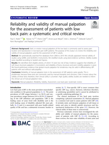
11distorted time series. This process scrambles up the physiological phase differences sothat they are irretrievably lost and can never be recovered. The method of mixing phasedifferences precludes meaningful physiological or clinical correlations since measuressuch as conduction velocity or synaptic rise or fall times can no longer be estimated dueto the average reference. Also, coherence methods such as “Directed Coherence” can notbe computed and more sophisticated analyses such as phase reset and phase shift andphase lock are precluded when using an average reference. The mixing together ofphase differences in the EEG traces is also a problem when using the Laplaciantransform and, similarly, reconstruction of EEG time series using IndependentComponent Analyses (ICA), also replaces the original time series with an altered timeseries that eliminates any physiological phase relationships and therefore is an invalidmethod of calculating coherence. One may obtain high reliability in test re-test measuresof coherence, however, the reliability is irrelevant because the method of computationusing an average reference or a Laplacian to compute coherence is invalid in the firstplace.As pointed out by Nunez (1981) “The average reference method of EEGrecording requires considerable caution in the interpretation of the resulting record” (p.194) and that “The phase relationship between two electrodes is also ambiguous: (p.195). As mentioned previously, when coherence is near unity then the oscillators aresynchronized and phase and frequency locked. This means that when coherence is toolow, e.g., 0.2, then the estimate of the average phase angle may not be stable and phaserelationships could be non-linear and not synchronized or phase locked.The distortions and invalidity of the average reference and Laplacian transformare easy to demonstrate using calibrated sine waves mixed with noise just as was done infigures 1 and 2.For example, figure three is the same simulation with a 300 phase shiftas used for coherence with a common reference as shown in figure 2. The top row iscoherence on the y-axis and the bottom row is the phase difference, the left column isusing the average reference and the right column is the Laplacian. It can be seen infigure 3 that coherence is extremely variable and does not decrease as a linear function ofsignal-to-noise ratio using either the average reference nor the Laplacian montage. It can

12also be seen in figure 3 that EEG phase differences never approximate 30 degrees and areextremely variable at all levels of the signal-to-noise ratio.Fig. 3-. Left top is coherence (y-axis) vs signal-to-noise ratio (x-axis) with a 300 phase shift as shown infigure 2 using the average reference. The left bottom is phase differences in degrees in the y-axis and thex-axis is the signal-to-noise ratio using the average reference. The right top graph is coherence (y-axis) vssignal-to-noise ratio (x-axis) using the Laplacian montage. The right bottom is phase difference on they-axis and signal-to-noise on the x-axis using the Laplacian montage. In both instances, coherence dropsoff rapidly and is invalid with no linear relationship between signal and noise . The bottom graphs showthat both the average reference and the Laplacian montage fails to track the 300 phase shift that was presentin the original time series. In fact, the phase difference is totally absent and unrepresented when using anaverage reference or a Laplacian montage and these simulations demonstrate that the average referenceand the Laplcain montage are not physiologically valid because they do not preserve phase differences orthe essential time differences on which the brain operates.The results of these analyses are consistent with those by Rappelsberger, 1989who emphasized the value and validity of using a single reference and linked ears inestimating the magnitude of shared or coupled activity between two scalp electrodes.The use of re-montage methods such as the average reference and Laplacian sourcederivation are useful in helping to determine the location of the sources of EEG of

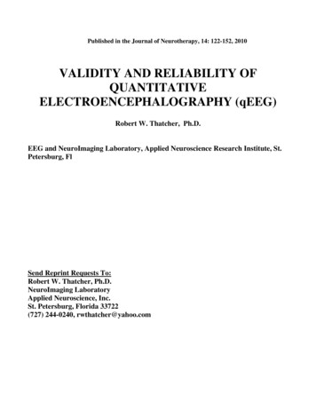
13different amplitudes at different locations. However, the results of this analysis whichagain confirm the findings of Rappelsberger, 1989 showed that coherence is invalid whenusing either an average reference or the Laplacian source derivation. This sameconclusion was also demonstrated by Korzeniewska, et al (2003) and Essl andRappelsburger (1998); Kamiński and Blinowska (1991); Kamiński et al (1997).The average reference and the Laplacian transform also distort measures of phasedifferences which is also easy to demonstrate by using calibrated sine waves. Forexample, a sine wave at Fp1 of 5 Hz and 100 uV with zero phase shift, Fp2 of 5 Hz and100 uV with 20 deg phase shift; F3 of 5 Hz and 100 uV with 40 deg phase shift; F4 of 5Hz and 100 uV with 60 deg phase shift; C3 of 5 Hz and 100 uV with 80 deg phase shift;C4 of 5 Hz and 100 uV with 100 deg phase shift; P3 of 5 Hz and 100 uV with 120 degphase shift; P4 of 5 Hz and 100 uV with 140 deg phase shift; O1 of 5 Hz and 100 uVwith 160 deg phase shift and O2 of 5 Hz and 100 uV with 180 deg phase shift andchannels F8 to Pz 0 uV and zero phase shift. Figure 4 below compares the incrementalphase shift with respect to Fp1 using Linked Ears common reference (solid black line),the Average Reference (long dashed line), and the Laplacian (short dashed line). This isanother demonstration of how a non-common reference like the average reference and theLaplacian scramble phase differences and therefore caution should be used and only acommon reference recording (any common reference and not just linked ears) is the onlyvalid method of relating phase differences to the underlying neurophysiology, e.g.,conduction velocities, synaptic rise times, directed coherence, phase reset, etc.The analyses of the average reference and Laplacian to compute coherence shouldnot be interpreted as a blanket statement that all of qEEG is invalid. On the contrary,when quantitative methods are properly applied and links to the underlyingneuroanatomy and neurophysiology are maintained then qEEG analyses are highlyreliable and physiologically valid. The lesson is that users of this technology must betrained and the use of calibration sine analyses should be readily available so that theusers of qEEG can test basic assumptions themselves.

14Fig. 4 – Demonstration of distortions in phase differences in a test using 20 degincrements of phase difference with respect to Fp1. The solid black line is using aLinked Ears common reference which accurately shows the step by step 20 deg.Increments in phase difference. The average reference (dashed blue line) and theLaplacian (dashed red line) significantly distort the phase differences.Validity by Hypothesis Testing and qEEG Normative Data BasesThe Gaussian or Normal distribution is an ideal bell shaped curve that provides aprobability distribution which is symmetrical about its mean. Skewness and kurtosis aremeasures of the symmetry and peakedness, respectively of the gaussian distribution. Inthe ideal case of the Gaussian distribution skewness and kurtosis 0. In the real world ofdata sampling distributions skewness and kurtosis 0 is never achieved and, therefore,some reasonable standard of deviation from the ideal is needed in order to determine theapproximation of a distribution to Gaussian.The primary reason to approximate"Normality" of a distribution of EEG measures is that the sensitivity (i.e., true positiverate) of any normative EEG database is determined directly by the shape of the sampling

15distribution. In a normal distribution, for example, one would expect that approximately5% of the samples will be equal to or greater than 2 standard deviations andapproximately 0.13 % 3 SD. (Hayes, 1973; John, 1977; John et al, 1987; Prichep, 2005;Thatcher et al, 2003a; 2003b).A practical test of the sensitivity and accuracy of a database can be provided bycross-validation. There are many different ways to cross-validate a database. One is toobtain independent samples and another is to use a leave-one-out cross-validation methodto compute Z scores for each individual subject in the database. The former is generallynot possible because it requires sampling large numbers of additional subjects who havebeen carefully screened for clinical normality without a history of problems in school,etc.The second method is certainly possible for any database.Gaussian cross-validation of the EEG database used to evaluate TBI was accomplished by the lattermethod in which a subject is removed from the distribution and the Z scores computedfor all variables based on his/her respective age matched mean and SD in the normativedatabase. The subject is placed back in the distribution and then the next subject isremoved and a Z score is computed and this process is repeated for each normal subjectto obtain an estimate of the false positive hit rate. A distribution of Z scores for each ofthe EEG variables for each subject was then tabulated.Figure 5 is an example of theGaussianFig. 5 – Example of Gaussian Cross-Validation of EEG Normative Database (from Thatcher et al,

162003).distributions of the cross-validated Z scores of 625 subjects from birth to 82 years of ageused in a normative EEG database (Thatcher et al, 2003a).T ab l e I: C ro ss Va l i dat i on of E EG N or ma t ive D at abas e ( f ro m Th atc he r et a l ,2 003 ) .Measure% 2 SD2.58Delta Amplitude Asym.2.29Theta Amplitude Asym.2.71Alpha Amplitude Asym.2.68Beta Amplitude Asym.1.99Delta Coherence2.22Theta Coherence2.55Alpha Coherence2.20Beta Coherence0.89Delta Phase †1.61Theta Phase †1.61Alpha Phase †2.83Beta Phase †4.15Absolute Power †4.09Relative Power4.23Total Power †2.58Average† Data was logged transformed% 2 SD% 3 SD% 3 60.180.100.230.130.240.030.1200.040.14Table I shows the results of a Gaussian cross-validation of the 625 subjects i

is greater than 0.9 reliable with as little as 40 second epochs and remains stable with high test re-test reliability over many days and weeks. Predictive validity of qEEG is established by significant and replicable correlations with clinical measures and accurate predictions of outcome and performance on neuropsychological tests.