Transcription
Chapter 2. Economic Analysis of Water ResourcesDaene C. McKinney2.1 Cost – Benefit Analysis2.1.1 Choosing Among Feasible AlternativesEconomic analysis, or the understanding and prediction of decision making under conditions ofresource scarcity, plays a major role in the planning, design and management of sustainablewater resource systems. Allocation of water among competing uses to obtain an optimum valuein terms of market or welfare measures is one of the main problems of water resources planners.Price theory is very relevant where markets are operating efficiently, whereas welfare economicsseeks to maximize human welfare in situations where desirable social gains and undesirablesocial costs are not fully accounted for in a profit maximizing, market economy (North, 1985).Price theory and welfare economics tend to focus on static analyses of projects, whereas,financial analysis considers the time value of investments and decisions. In this section, we willconsider some aspects of financial analysis.Choice is governed by economic and financial feasibility and acceptability with respect to socialand environmental impacts. Here we want to consider investment analysis which serves as aguide for allocating resources between present and future consumption. The process consists of:Identifying alternatives to be considered;Predicting the consequences resulting from these alternatives;Converting the consequences into some commensurable units (e.g., ’s); andChoosing among the alternativesOne project may produce one type of output, while another project produces another kind ofoutput. In order to compare the projects and make investment decisions, common units must beused to express the outputs of each alternative before any comparison can be made. Monetaryunits are the most commonly used units.Some projects will provide outputs in the near future and other projects may delay outputs for anappreciable time or distribute them uniformly over the project lifetime. Outputs today do nothave the same value as outputs tomorrow and the following observations are appropriate: Investors often prefer early return on investments since it provides them with moreflexibility in making future investment decisions;Benefits and costs at different times should not be directly compared or combined, sincethey are not in common units;Future benefits and costs must be multiplied by a factor that becomes progressivelysmaller for times further into the future. This multiplicative factor is called the discountrate and it has a great impact on the alternative selected;Future benefits and costs are given more weight with lower discount rates and less weightwith higher discount rates; and1
Committing resources to one project may deny the possibility of investing in some otherproject. This brings up the question of opportunity costs, or what must be foregone inorder to undertake some alternative.One should always keep in mind that different points of view may be adopted in analyzingalternatives, e.g., project sponsors; people in a specific area or region; and an entire nation. Eachpoint of view may value benefits and costs differently and even define items differently (i.e., oneperson’s cost may be another person’s benefit.).2.1.2 Cost-Effectiveness AnalysisA program is cost-effective if, on the basis of life cycle cost analysis of competing alternatives, itis determined to have the lowest costs expressed in present value terms for a given amount ofbenefits. Cost-effectiveness analysis is appropriate whenever it is unnecessary or impractical toconsider the dollar value of the benefits provided by the alternatives under consideration. This isthe case whenever (i) each alternative has the same annual benefits expressed in monetary terms;or (ii) each alternative has the same annual affects, but dollar values cannot be assigned to theirbenefits. Analysis of alternative defense systems often falls in this category (OMB, 1992).2.1.3 Benefit-Cost AnalysisFinancial benefit-cost analysis evaluates the effect of a project on the water sector or utility byproviding projected balance, income, and sources and applications of fund statements (ADB,2005). This can be distinguished from economic benefit-cost analysis which evaluates the projectfrom the viewpoint of the entire economy. In financial benefit-cost analysis, which we willconsider here, the unit of analysis is the project and not the entire economy nor the entire watersector or utility. Therefore, it focuses on the additional financial benefits and costs to the watersector, attributable to the project.Benefit – Cost Analysis is a systematic quantitative method of assessing the desirability ofgovernment projects or policies when it is important to take a long view of future effects and abroad view of possible side-effects (OMB, 1992). Both costs and benefits of a project must be measured and expressed in commensurableunits;It is the main analytical tool used to evaluate water resource and environmental decisions;Benefits of an alternative are estimated and compared with the total costs that societywould bear if that action were undertaken; andViewpoint is important - some groups are only concerned with benefits, others areconcerned only with costsIn benefit – cost analyses, any costs and benefits that are unaffected by which alternative isselected should be neglected. That is, the differences between alternatives need only beconsidered.2
Estimates of benefits and costs are typically uncertain because of imprecision in both underlyingdata and modeling assumptions. Because such uncertainty is basic to many analyses, its effectsshould be analyzed and reported (OMB, 1992). Uncertainty may exist in: objectives, constraints,public response, technological change, or extreme events and recurrence.2.1.3.1 Interest Rate CalculationsConsider investing 100 at a rate of 5%. At the end of one year the value of the investmentwould be:F1 100(1 0.05) 105(2.1.1)Similarly, at the end of 2 years, the value would beF2 105(1 0.05) 100(1 0.05) 2 110.25(2.1.2)or, generalizing this, we have at the end of t years that an initial investment of P would beworthFt P (1 i )t(2.1.3)Put another way, a single payment of Ft available t years in the future is worthP Ft(1 i )t(2.1.4)and a series of (not necessarily equal) payments Ft available t years in the future is worthP TFt (1 i)t 1t(2.1.5)Example 1. Assume that an initial investment of 50 disbursement at t 0 is required and thatthis will result in 200 receipt at t 1 year and 150 receipt at t 2 years with an interest rate of7% annually (see figure).3
200 150120 50Figure 2.1. Cash flow diagramWhat is the Present Value, P, of the given cash flow?P C Ft (1 i) t C F1 (1 i) 1 F2 (1 i) 2(2.1.6)tFill in the blanks:P () (P () ) ()What is the Future Value of the given cash flow at the end of year 2?F C (1 i) 2 F1 (1 i) 1 F2(2.1.7)Fill in the blanks:F () (F () ) ()2.1.4 Financial AnalysisFinancial analyses use cash flow analysis and discounting techniques in benefit-cost analyses tomaximize the rate of return to capital. Capital is the limiting factor here and maximizing profit isnot necessarily achieved. The basic principle is that an investment will be made if revenues inthe future will repay the cost at a positive rate of interest (North, 1985).The standard criterion for deciding whether a government program can be justified on economicprinciples is net present value -- the discounted monetized value of expected net benefits (i.e.,benefits minus costs). Net present value is computed by assigning monetary values to benefitsand costs, discounting future benefits and costs using an appropriate discount rate, andsubtracting the sum total of discounted costs from the sum total of discounted benefits.Discounting benefits and costs transforms gains and losses occurring in different time periods to4
a common unit of measurement. Programs with positive net present value increase socialresources and are generally preferred. Programs with negative net present value should generallybe avoided (OMB, 1992).The process proceeds as: Define each alternative and predict their consequencesPlace monetary value on consequencesSelect a discount rateConvert time streams of benefits and costso Construct cash flow diagramso Convert values of costs and benefits at one date to equivalent values at the present (oranother convenient) time.NBt Bt Ct(2.1.8)where NBt Net benefits at time t, Bt benefits at that time, and C t costs at that time. ThePresent Value of net benefits isTP NBtt 1 (1 i )t(2.1.9)Often it is convenient to convert a present value to an equivalent annual value. For this we canuse the Capital Recovery Factor (CRF)CRFT i(1 i)T(i 1)T 1Then the equivalent annual value is(2.1.10)A P CRFT(2.1.11)2.1.5 Discount RateIn order to compute net present value, it is necessary to discount future benefits and costs. Thisdiscounting reflects the time value of money. Benefits and costs are worth more if they areexperienced sooner. All future benefits and costs, including nonmonetized benefits and costs,should be discounted. The higher the discount rate, the lower is the present value of future cashflows. For typical investments, with costs concentrated in early periods and benefits following inlater periods, raising the discount rate tends to reduce the net present value (OMB, 1992).The discount rate measures the rate at which current consumption will be sacrificed to ensure5
consumption (production) later. Greater sacrifices mean more resources can be devoted to futureproduction. Alternatives discount rates include: Zero;Interest paid to borrow funds for project financing;Internal rate of return;Market interest rate for risk free investments -- Interest on recently issued governmentbonds having a maturity date approximately equal to the project lifeMost productive investments (opportunity cost of capital) -- If funds were committed to aproject yielding the highest rate of return first, then to subsequent projects in order of rateof return, the IRR of the last project selected before funds run out is the MIRRInterest paid on borrowed funds for governments using bond financingUS federal practice (Senate Doc. 97, 1962) -- “Average rate of interest payable by the USTreasury on interest-bearing marketable securities outstanding at the end of the fiscalyear preceding computation which had terms to maturity of 15 years or more”. Index.html for current and historicrates.2.1.6 ExamplesExample 2. (after Linsley, et. al., 1979) Two alternative plans are considered for a section ofan aqueduct. Plan A uses a tunnel, and Plan B uses a lined canal and steel flume. Both plansyield the same revenues over the life of the project. The interest rate is 6 % per year and thestudy period is 100 years.Table 2.1. Information for Example 1.Plan APlan BTunnelCanalCanal lining FlumeLife100 yr100 yr20 yr50 yrFirst cost 450,000 120,000 50,000 90,000Annual O&M cost 4000 10,500Compare the equivalent annual costs of the two plansCRF i (1 i ) N(i 1) N 1(2.1.12)where i 0.06 and N 20, 50, and 100 years6
Table 2.2. Calculations for Example 1.Plan ACapital recovery cost for the tunnelAnnual maintenance costTotal annual cost 450,000 x 0.060177 27,080 4,000 31,080Plan BCapital recovery cost for canal 120,000 x 0.060177 7,221Capital recovery cost for canal lining 50,000 x 0.087184 4,359Capital recovery cost for flume 90,000 x 0.063444 5,710Annual maintenance cost 10,500Total annual cost 27,790Total investment is 450,000 and 260,000, respectively, for the two projects. Even though theannual O&M costs are lower for Plan A, the annual cost comparison tells us that the extrainvestment is not justified. Thus Plan B should be selected.Where the capacity of the project is to be determined, we simply determine the project with themaximum net benefits (difference of benefits over costs). That is:Max NB( x) B( x) C ( x)(2.1.13)where x is the capacity of the project. ThusdB ( x) dC ( x) dxdx(2.1.14)dB ( x) 1dC ( x)(2.1.15)orThat is, we increase the capacity up to the point where the marginal (incremental) benefits justexceed the marginal (incremental) costs and then stop.Example 3. (after North, 1985, Ex. 5-1) A flood control district can construct severalalternative control works to alleviate flooding. These alternatives include the construction of damA, dam B, and a system of levees C. Each of these works can be built to function alone ortogether with any other or all other projects. Thus we have a possibility of the followingcombinations: ABC, A, B, C, AB, AC, and BC. The life of each dam is 80 years and the life ofthe levee system is 60 years. The cost of capital is 4% . Information on total investment,operation and maintenance costs, and average annual flood damages is given in the table. Whichflood control undertaking is the most economical?7
ProjectABCABACBCABCDo nothingTable 2.3. Flood Control Project DataTotal InvestmentAnnual OperationAverage Annual(million )and MaintainenceFlood Damages(thous. )(million 52700.25002.00The annual investment costs can be computed for each alternative by multiplying the investimentcost by the appropriate capital recovery factor:CRFT i(1 i)T(i 1)T 1(2.1.16)where T 80 years for dams and 60 for levees, respectively.ProjectABCABACBCABCTable 2.4. Flood Control Project ntOperation and( mln)CostsMaintainence( mln)( 0.270TotalAnnual Cost( mln)0.3410.2890.3650.6300.7060.6540.995The Incremental Benefit – Cost Ratio Method compares the additional benefit to the cost ofany alternative compared to other alternatives to find the solution. The procedure is:1. Discard any alternative with B/C 12. Rank order the alternatives from lowest to highest cost3. Compute the incremental benefit - cost ratio for the contender versus current bestalternative. If that ratio is greater than 1, contender becomes current best.4. Repeat until all alternatives have been tested. Final current best is preferred alternative.8
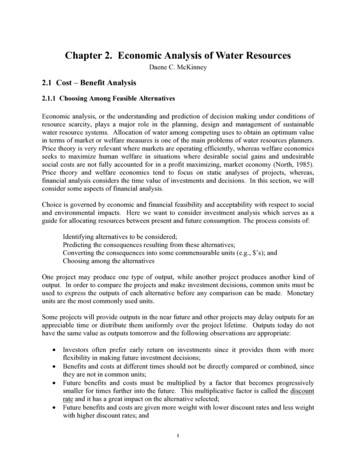
Table 2.5. Further Flood Control Project CalculationsComparison ΒB AC AAB CBC CAC CABC CProjectBACABBCACABCBenefits( mln)0.70.91.31.11.51.61.75Cost( 2.643.561.752.292.271.76ΔB( mln)0.70.20.4-0.20.20.30.45ΔC( usion2.43.817-0.750.690.880.71 ΒA BC AC ABC BCC ACC ABCExample 4. (after Mays and Tung, Example 2.2.1) Determine the optimal scale ofdevelopment of a hydroelectric project using benefit – cost analysis. Various alternative sizeprojects and corresponding benefits are shown in the table below.Table 2.6. Hydropower Project DataScale Benefits CostsNet(MW)BCBenefits( mln) ( B-Cmln)( 050.050.00.0The following figures show plots of the (1) project benefits and costs versus capacity, and (2)project benefits versus costs. Using a marginal analysis we find that the optimal capacity is 100MW. The following table shows the incremental benefit – cost ratio method to find the samesolution as before.Table 2.6. Incremental Cost-Benefit Analysis for Hydropower ProjectIncrementalIIIIIIIVVVIVIIVIIComparisonScale (MW)B( mln)C( mln)ΔB( mln)ΔC( mln)ΔB/ΔCConclusion II IIII IIIII IVIV VV VIV VIIV .291.110.890.850.72 III IIII IIIV IIIV IVVI VVII VVIII V9
50BenefitsCosts45Benefits or Costs ( mln)40CostsBenefits3530Max ( B - C )25201510406080100120140160180200Capacity (MW)Figure 2.2. Project benefits and costs versus capacity.6050Benefits ( mln)40B C line30Max NB20100010203040Costs ( mln)Figure 2.3. Project benefits versus costs.105060
Example 5. (after James and Lee, p. 33) The project with the highest benefit-cost ratio maynot always be the preferred alternative. Consider a project whose benefits equal 3 units andwhose costs equal 1 unit and which has an increment of investing an additional 4 units toincreate benefits to 10 units. The smaller project has a benefit-cost ratio of 3, while the largerone has a ratio of 2. Because the incremental benefit-cost ratio is 1.75, the larger investmentshould be chosen even though it has a smaller individual benefit cost ratio.Table 2.7. Incremental Cost-Benefit Analysis for Example 5IncrementalBC Β/ CA 3 1B 10 532ΔBΔCΔB/ΔCConclusion371431.75A preferredB preferred to AExample 6. (after Thuesen, Fabrycky, and Thuesen, pp. 285-287 with correction) Supposethat four projects have been identified for providing recreational facilities for a Lower ColoradoRiver Authority facility. The equivalent annual benefits, equivalent annual costs, and benefitcost ratios are given in Table 2.8. Inspection of the benefit-cost ratios might lead one to selectAlternative B because the ratio is a maximum. Actually this choice is not correct. The correctalternative can be selected by applying the incremental benefit-cost method where the additionalincrement of investment is desirable if the incremental benefit realized exceeds the incrementaloutlay. The alternatives must be arranged in order of increasing outlay. Thus, the alternativewith the lowest initial cost should be first, the alternative with the next lowest initial cost second,and so forth.Table 2.8. Incremental Cost-Benefit Analysis for Example 6ABCDB(1000 )C(1000 )Β/ ng these rules to the alternatives indicates that Alternative A and not Alternative B ifs themost desirable alternative.Table 2.9. Incremental Cost-Benefit Analysis for Example 6IncrementalBCΒ/ CΔBΔCD 95 50.0 1.90 9550B 167 79.5 2.10 72 29.5C 115 88.5 1.30 -52.09A 182 91.5 1.99 151211ΔB/ΔCConclusion1.902.44-5.771.25D preferredB preferred to DB preferred to CA preferred to B
2.2 Demand for Water2.2.1 IntroductionConsumers purchase goods produced by firms. They have preferences for some goods overothers and they choose purchases from a set of feasible options. A utility function u(x) is anumerical representation of consumer preferences. If one bundle of goods is preferred to anotherbundle, then it must have a higher utility. Indifference curves are the level sets of a utilityfunction (see Figure 2.2.1.1).x2u(x1,x2)Betterbundle areaIndifference curvedx2dx1x2*Budget lineWorsebundle areaSlope MRS12x1*x1Figure 2.4. Indifference curve.Consider the case when there are 2 goods to choose from, x1 and x2. If the consumer changesconsumption by a small amount (dx1, dx2 ) but keeps utility constant, say at level uo, thendu ( x) whereMU i u udx1 dx2 0 x1 x2 u xi(2.2.1)i 1,2(2.2.2)is the marginal utility of good i or the change in utility due to a small change in xi. We can write12
dx 2 MU1 MRS12dx1 MU 2(2.2.3)where MRSij is the marginal rate of substitution of good i for good j, that is, the rate at which aconsumer can substitute good i for good j.2.2.2 Consumer’s ProblemConsumers attempt to choose the best bundles of goods that they can afford. If there are Kgoods, whose quantities are represented by the vector x ( x1,!, xK ) , available forconsumption with unit prices p ( p1,!, pK ) and the total amount of money available to theconsumer is m, then the consumer must make choices between goods according to a budgetaryconstraintKp T x pk xk mk 1(2.2.4)Consider the case of 2 goods. The budgetary constraintp1x1 p2 x2 m(2.2.5)separates the decision space into two regions: (1) a region containing those combinations ofgoods whose purchase would exceed the budget; and (2) a region where those combinations thatwould not exceed the budget (See Figure 2.2.2.1). The slope of the budget line ( pi / p j ) is therate at which the market will substitute good i for good j. Now, in the general case of K goods,the consumer is faced with the problemMaximize u ( x )subject top x m(2.2.6)x 0That is, the consumer tries for maximize utility while satisfying the budget constraint. Now,assume that the budget constraint (Eq. 2.2.2.4) holds as an equality (all funds are expended orone of the goods is actually a savings account) and that the levels of consumption are all positive.Then we have the classical programming problem with a Lagrangian functionL( x, λ ) u ( x ) λ (m p x )K u ( x ) λ m p k xk k 1 (2.2.7)13
x2Unaffordablebundlesm/p2Budget linep1x1 p2x2 mSlope -p1/p2Affordablebundlesm/p1x1Figure 2.5. The consumer’s budget setThe first-order optimality conditions for this problem are L u 0 λp k , xk xkk 1,., K(2.2.8)K L 0 m pk xk λk 1(2.2.9)The first condition (Eq. 2.2.2.6) says that the ratio of the marginal utility to price is constant forall inputsMU k pk u x k λpkk 1,., K(2.2.10)orMU1 MU 2MU K . λp1p2pK(2.2.11)That is, a consumer chooses purchases of goods such that the ratio of marginal benefit (marginalutility) to marginal cost (price) is equal among all goods. This ratio, with units of utility/ , is thevalue of the Lagrange multiplier (λ) which is also the ratio of the change in total utility for achange in income, or14
λ u m(2.2.12)If we write Eq. 2.2.2.9 for two goods, say goods i and j, we haveMU ip i MRS ijMU jpj(2.2.13)which says that the slope of the budget line will equal the slope of the indifference curve. or theratio of the marginal utilities of any two goods equals the ratio of their prices.x2Indifference curveslope MRS12Optimal choiceMRS12 p1/p2Budget lineslope -p1/p2x2*Increasingutilityx1*x1Figure 2.6. The consumer’s problem and solution.2.2.3 DemandThe optimal solution to the consumer’s problem depends on income and prices so solving theproblem (Eq. 2.2.2.3 and 2.2.2.4) results in an optimal level of consumption x * x * ( p, m)which is a function of the prices and the available income. This is the demand function. Atypical demand function is shown in Figure 2.2.3.1. Often the inverse demand function,p p(x*, m), is used in analyses; this is simply the inverse of the demand function or price as afunction of quantity and income. Market demand is the aggregation of all of the individualconsumers’ demands. Market demand depends on prices and the distribution of income in theeconomy.15
Price, pDemand curvex(p,m)Quantity, xFigure 2.7. Typical demand curve.2.2.4 Willingness-to-PayDemand is only real (or "effective") when it is accompanied by willingness to pay, in cash orkind, for the goods or services offered (Evans, 19921). The value of a good to a person is whatthat person is willing, and able, to sacrifice for it (willingness-to-pay). How do we measure whata person is willing to pay for a good? Assume that a farmer has no irrigation water forproduction of a particular crop, but desires to purchase some water. If one unit of water becameavailable, how much would the farmer be willing to pay to obtain that unit of water, rather thanhave no water at all? Suppose the farmer is willing to pay 38 for this first unit (see Figure2.4.1) even though (s)he would prefer to pay less. Now, suppose that the farmer is willing to pay 26 for a second unit of water. Further, suppose that the farmer is willing to pay 17 for a thirdunit. According to the figure, at p* 10 per unit, the farmer would purchase 4 units of waterfor a total cost of 40, but (s)he would have been willing to pay 93 for that water. Thus, thefarmer receives a surplus of 53 (consumer surplus) when purchasing the 4 units of water.Evans (1992) suggests three ways of determining willingness-to-pay from direct information inother, similar, situations and from survey information: Indirect method, involves analyzing what others in similar circumstances to the targetpopulation are already paying for services;Direct method (or contingent valuation method), involves asking people to say what theywould be prepared to pay in the future for improved services; andProxy measures, e.g., use of case studies of water vending to provide indicators ofwillingness to pay.1 Evans, Phil, Paying the Piper: An overview of community financing of water and sanitation, Occasional Paper 18,IRC International Water and Sanitation Centre, The Hague, The Netherlands, April 199216
Price, p4038WTP 93302620CS 531712p* 10Cost 4012345Quantity, xFigure 2.8. Willingness-to-pay for each additional unit of water.If we assume that fractional amounts of a unit of a good can be purchased, then we obtain acontinuous graph. Marginal willingness-to-pay is the height of the curve. Total willingness-topay is the sum of the heights of the rectangles between the origin and the particular consumptionlevel, x, of interest. In the case of the continuous curve, willingness-to-pay is the area under thecurve from the origin and the particular consumption level of interest and this represents thegross benefit of purchasing this amount of the good. The net-benefit from this purchase is thewillingness-to-pay minus the cost orx*NB p(η , m)dη p * x *0(2.2.14)which is termed the consumer’s surplus.17
Price, pConsumer surplusx* p ( x, m) dx p * x *0p*Cost p*x*x*Quantity, xFigure 2.9. Willingness-to-pay curve.Measuring benefit of water use in this manner requires that we can derive the demand curve forthe water used for a particular purpose. For marketed commodities with available informationon prices and quantities we can: (1) derive a demand curve, (2) quantify willingness-to-pay, and(3) use WTP to represent benefits. However, in many cases market prices may not exist,demands may not be revealed, and the change in benefits over time may be extremely uncertain.Examples include (1) the benefits of preserving space for recreation, and (2) the benefits derivedfrom damages prevented due to pollution controls. If the physical damages of pollution can beidentified and estimated, then a monetary value may be placed on them (for an example ofapplying this to the Aral Sea basin, see Anderson, 1997). Sometimes it is possible to surveypeople to determine their willingness-to-pay for different environmental assets such asenvironmental preservation, damage reductions, and lower risks. From these survey results wemay be able to infer the valuation of the assets. Indeed, we may also be able to infer these valuesfrom related markets where values are observable.The value of municipal water at its source minus any water utility costs is represented by theconsumers' surplus. The area under the demand curve for an increment from x1 to x2 is (Gibbons,1986)Area px2χ x2x 1 1 β xβ xβ 1 2β 1ε(2.2.15)18
2.2.5 Elasticity (of demand)The price elasticity of demand is a measure of how responsive consumers are to changes in price.The slope of the demand function x * x * ( p, m) isslope dxdp(2.2.16)This quantity depends on the units used to describe the inputs and price. If we normalize thisfunction, we obtain the price elasticity of demandelasticity ε dxdpxp(2.2.17)Consider the following example adapted from Merrett (1997). Table 2.7 shows the quantity ofwater demanded for different prices along with the price elasticity of water at variousincrements. Figure 2.10 plots the demand function for water and illustrates the ranges of elasticand inelastic behavior. Merrett (1997) proposes a cubic form for the demand functionp ax 3 bx 2 cx d(2.2.18)where a 0, b 0, c 0, and d 0. He points out, at low quantities, higher prices for water havelittle effect due to the intense need for the water. Similarly, at low quantities, higher prices forwater have little effect due to the abundance of water. In the middle quantities, changes in priceproduce significant changes in the quantity of water demanded.Price elasticity of municipal water demand was estimated (Gibbons, 1986) and in-house wateruse was found to be price-inelastic ( -0.23), while sprinkling use was found to be more elasticand differ between the Eastern US ( -1.6) and the Western US ( -0.7).19
Table 2.7. Price Elasticity of Water (adapted from Merrett, 1997)QuantityPriceΔQΔPε33(m /month)(per m 625002300-10.21280016ε 1, elastic P, Q, TR54Price, pε 1, inelastic P, Q32ε 1, inelastic P, Q, TR100500100015002000Quantity, xFigure 2.10. Demand function for water.2025003000
2.2.6 Water Values in the USTable 2.8 shows data on the value of water for various uses within the United States [Frederricket al. (1996).Table 2.8. National Water Value by Use ( /af) [Frederrick et al. (1996)]AverageMedianMinMaxInstreamWaste 54001228Industrial28213228802Thermo Power3429963Domestic1949737573Table 2.9 shows data on the value of water for recreations and fish & wildlife uses within theUnited States and Table 2.2.6.3 shows the value of water use in irrigated agriculture.Table 2.9. Water Values for Recreation/F&W Habitat ( /af) [Frederrick et al. (1996)]AverageMedianMinMaxFishing3450158Wildlife Refuge246144Fishing & Whitewater1042150563Whitewater9954Shoreline Recreation191917221
Table 2.10. Water Values by Crop ( /af) [Frederrick et al. 339Beans5858Carrots550550Corn9198Cotton114103Grain r5358Soybeans121127Sugar 2.3 Supply of Water2.3.1 IntroductionFirms produce outputs from various combinations of inputs. The objective of a firm is t
2.1.3 Benefit-Cost Analysis Financial benefit-cost analysis evaluates the effect of a project on the water sector or utility by providing projected balance, income, and sources and applications of fund statements (ADB, 2005). This can be distinguished from economic benefit-cost analysis which evaluates the project